SonicMoE: A Hardware-Efficient and Software-Extensible Blueprint for Fine-Grained MoEs
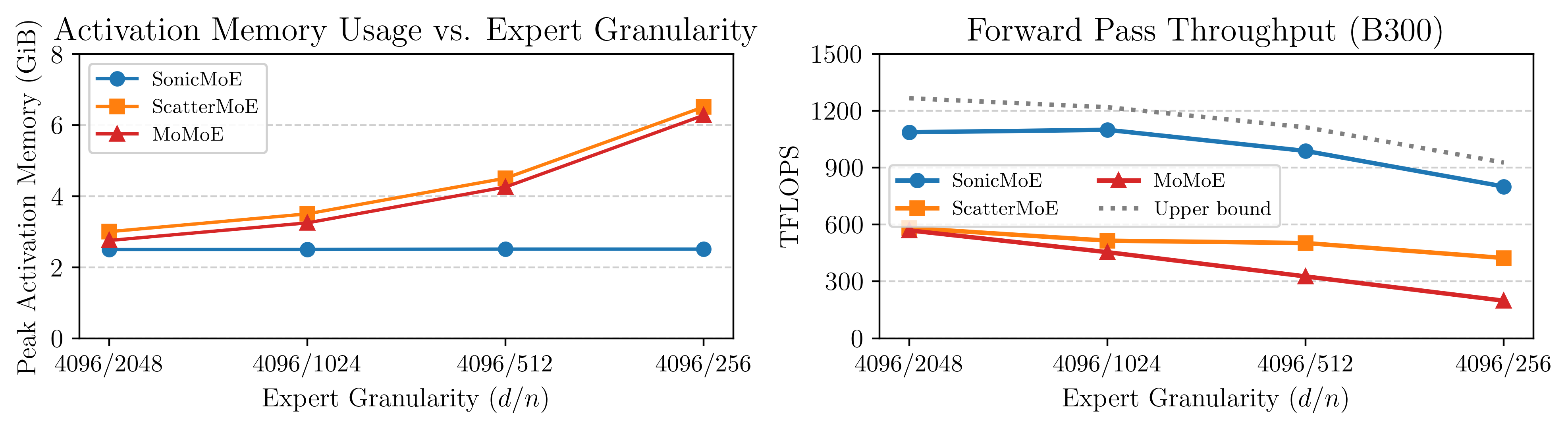
Figure: SonicMoE's per-layer activation memory footprint (left) stays constant even when expert granularity (embedding dimension / expert intermediate dimension) increases, and SonicMoE can achieve 1.87-4.04x relative speedup compared to existing MoE training kernels ScatterMoE and MoMoE.
SonicMoE now runs at peak throughput on NVIDIA Blackwell GPUs (B200/B300), in addition to its existing Hopper (H100) support. This blogpost walks through how we got there: an IO-aware algorithm that keeps activation memory independent of expert granularity, a unified software abstraction on QuACK that makes porting across GPU architectures straightforward, and the Blackwell hardware features we exploit to hide IO costs behind computation.
![]()

1. Opportunities and Pains of Fine-Grained MoEs
Mixture-of-Experts (MoE) models have become the dominant architecture for scaling language models without proportionally increasing compute. The appeal is straightforward: by routing each token to a small subset of \(K\) out of \(E\) expert networks, we get a model with hundreds of billions of parameters at the compute cost of a much smaller dense model. The training FLOP savings and quality improvements are well-established, but they come with hardware costs that grow worse as models become more fine-grained.
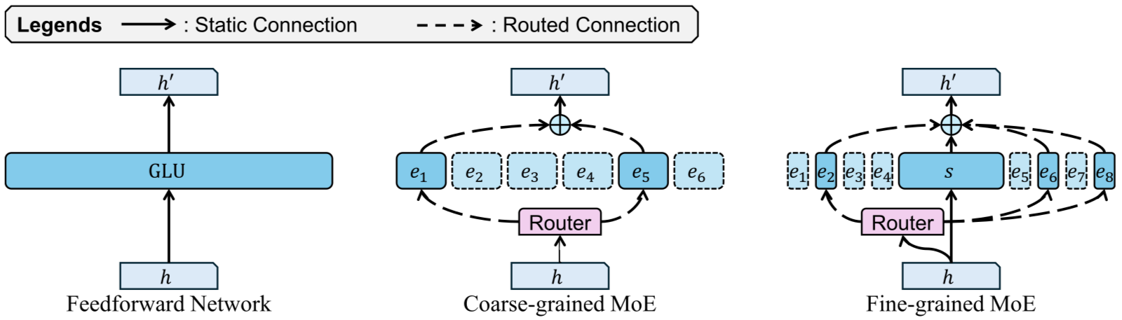
Figure: fine-grained MoE architecture [1]
Two architectural dimensions define how an MoE model trades off quality and efficiency.
-
Granularity (\(G = d/n\), where \(d\) is the model embedding dimension and \(n\) is each expert’s intermediate size) measures how small the experts are relative to the model width. A high-granularity (fine-grained) MoE has many small experts.
-
Sparsity (\(\rho = K/E\)) measures the ratio of experts activated per token.
MoE scaling laws, from controlled experiments (e.g. Krajewski et al. and Tian et al.) and recent open-source model scaling trends, consistently show that higher granularity and higher sparsity yield better model quality per FLOP: selecting more, smaller experts increases representational capacity, while sparser activation allows more total parameters within the same compute budget. Frontier open-source models reflect this clearly: Mixtral 8x22B, released in 2024, operated at \(G=0.38\) and \(\rho=0.25\), while recent models since 2025 like DeepSeek V3.2 (\(G=3.50\), \(\rho=0.03\)), Kimi K2.5 (\(G=3.50\), \(\rho=0.02\)), and Qwen3-Next-80B-A3B-Instruct (\(G=4.00\), \(\rho=0.02\)) have pushed both dimensions aggressively. Every new generation of frontier MoE is more fine-grained and sparser than the last.
However, the pursuit of granularity and sparsity comes with two painful hardware costs:
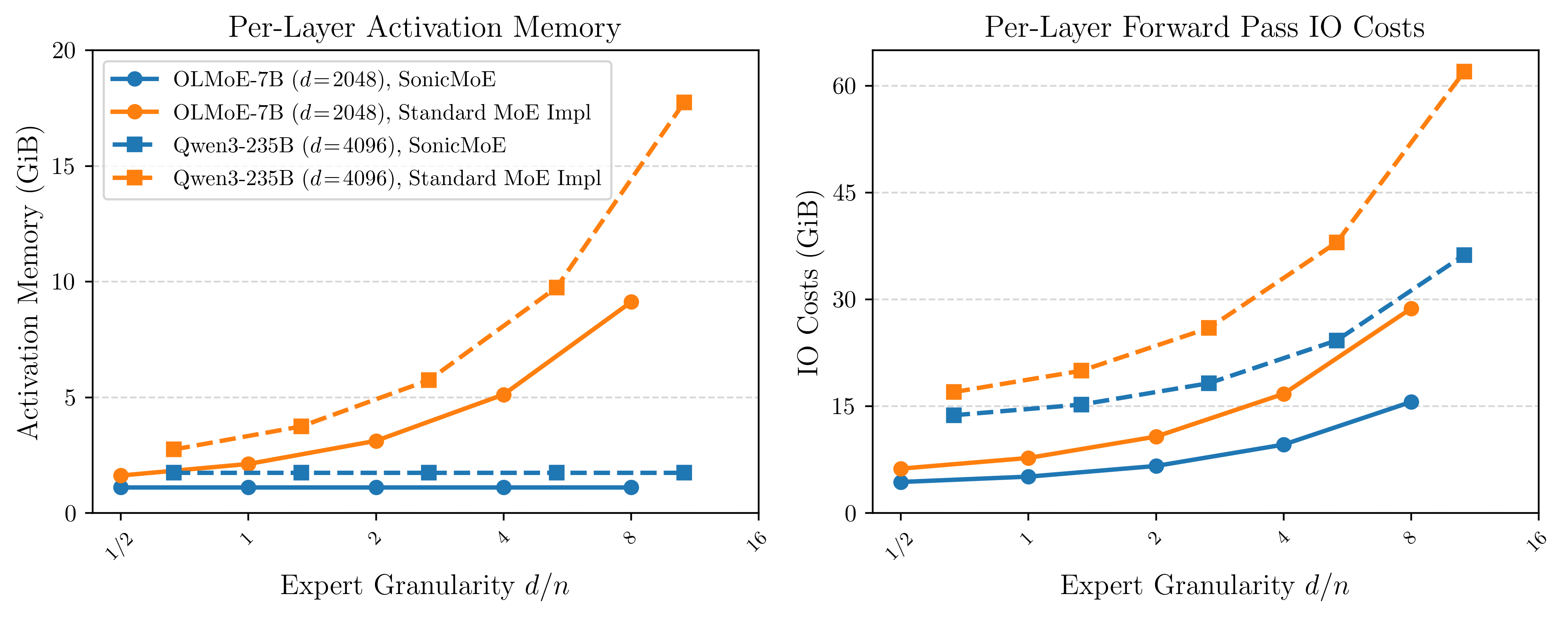
Figure: Per-layer activation memory (left) and forward IO costs (right) as expert granularity increases. We fix microbatch size as 32768 and each model's embedding dimension, then vary the expert intermediate size while keeping training FLOPs and parameter count constant.
Problem 1: Activation Memory Scales with Expert Granularity with Current Training Kernels.
During training, intermediate tensors must be cached for the backward pass. The total FLOPs of MoE forward and backward computation is \((6+12)TnKd\). For fixed \(T\) and \(d\), keeping FLOPs constant requires \(nK\) to stay constant. Increasing granularity means decreasing \(n\) and proportionally increasing \(K\). Any activation of size \(O(TKd)\) thus grows linearly with granularity.
For current MoE kernels like ScatterMoE and MoMoE, variables such as the down-proj output \(Y\) (size \(TKd\)) are cached for the backward pass, causing per-layer activation memory to grow linearly as experts become more fine-grained. Prior solutions such as MoMoE usually require a GEMM recomputation during backward to trade off activation memory for extra FLOPs. This raises the question:
Is it possible to achieve activation memory efficiency without extra FLOPs from GEMM recomputation?
Problem 2: IO Cost Scales with Expert Granularity and MoE Sparsity.
A GPU kernel’s runtime is determined by whichever resource is exhausted first: compute throughput (FLOP/s) or memory bandwidth (bytes/s). Arithmetic intensity as the ratio of FLOPs to HBM bytes transferred is the metric that determines in which regime a kernel operates. As the arithmetic intensity becomes higher, the kernel is likely to be compute-bound rather than memory-bound.
Assuming perfect load balancing and SwiGLU activation, the arithmetic intensity of a single expert’s forward pass is lower-bounded by:
\[\text{Arithmetic Intensity} = \frac{3}{\frac{2}{d} + \frac{2G}{d} + \frac{3}{T\rho}} = O\left(\min\left(\frac{d}{G}, T\rho\right)\right)\]where \(T\) is the number of tokens in a microbatch (\(T\rho\) is the average number of routed tokens per expert).
In this case, both increasing \(G\) and increasing MoE sparsity (decreasing \(\rho\)) would drive arithmetic intensity down. For example, Qwen3-Next-80B-A3B-Instruct would have an arithmetic intensity of 210 for a microbatch of 16K tokens, while an iso-param dense SwiGLU MLP would have an arithmetic intensity of 2570, 12× higher. In this regime, kernel runtime is dominated by the IO costs, not compute throughput.
For fine-grained and sparse MoEs, every expert’s GEMM problem shape is small enough such that the kernel falls into the memory-bound regime.
These IO costs will become a greater bottleneck in expert parallelism, as the intra- or inter-node network bandwidth are often much slower than HBM loading speed. SonicMoE currently focuses on the case of single GPU (EP degree=1), but the IO-aware algorithmic designs are transferable to expert parallelism.
MoE as Grouped GEMM
MoE computation is often implemented using Grouped GEMM. A Grouped GEMM is a batch of matrix multiplications with possibly different problem shapes. Following standard BLAS conventions used by CUTLASS, each GEMM computes \(C = AB\) where \(A \in \mathbb{R}^{M \times K}\) (activations), \(B \in \mathbb{R}^{K \times N}\) (weights), and \(C \in \mathbb{R}^{M \times N}\) (outputs).
In MoE, each expert usually receives a different number of tokens, and input tokens may need to be gathered from different positions, or they may already be contiguously packed by expert.
For the forward pass and backward activation gradient, we would need Grouped GEMM with input shapes that have constant \(N\) and \(K\) (embedding dimension and expert intermediate dimension) but different \(M\) (the number of routed tokens per expert). We call this varlen-M Grouped GEMM. (CUTLASS would describe it as Grouped GEMM with ragged M dimensions). For the backward weight gradient, we would reduce over token embeddings for each expert GEMM, in which \(M\) and \(N\) (embedding dimension and expert intermediate dimension) are fixed but the \(K\) dimension varies. We call this varlen-K Grouped GEMM.
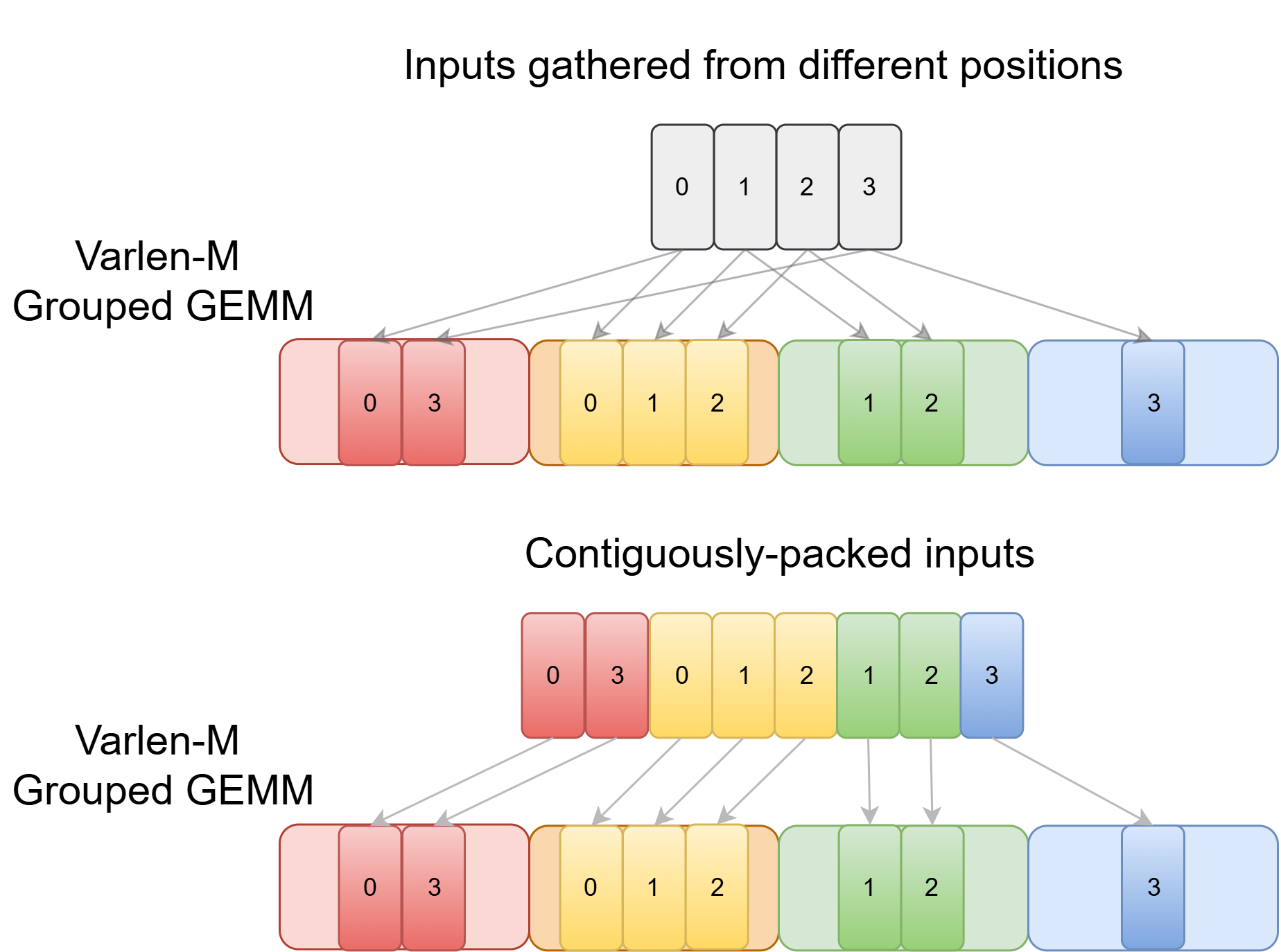
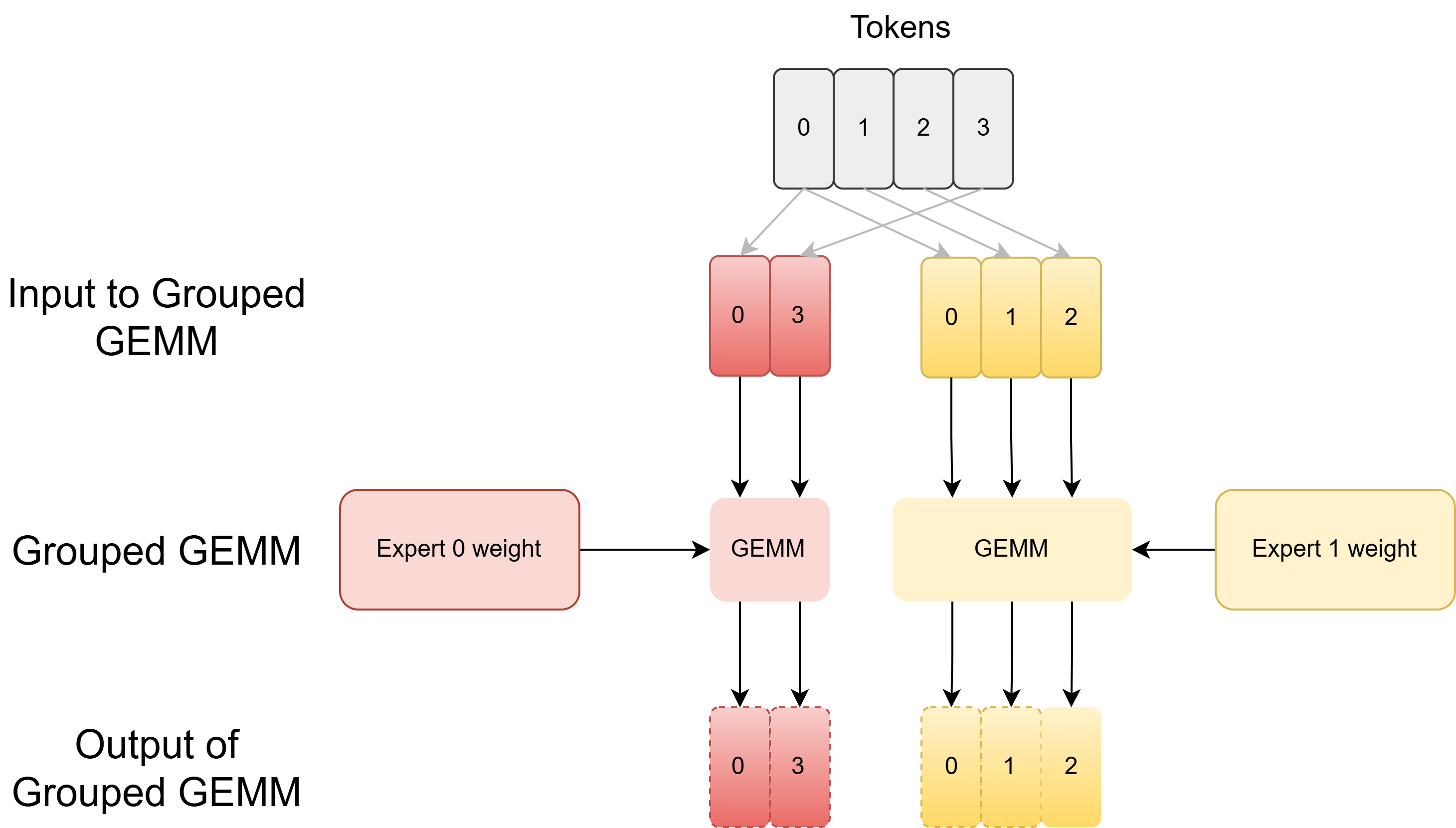
Left: Each expert gathers inputs from different positions on an input tensor (top) or reads a contiguous chunk on a grouped input array (bottom). Right: Illustration of using Grouped GEMM in MoE.
We can use varlen-M Grouped GEMM to build a standard MoE forward pass as demonstrated in the following code snippet.
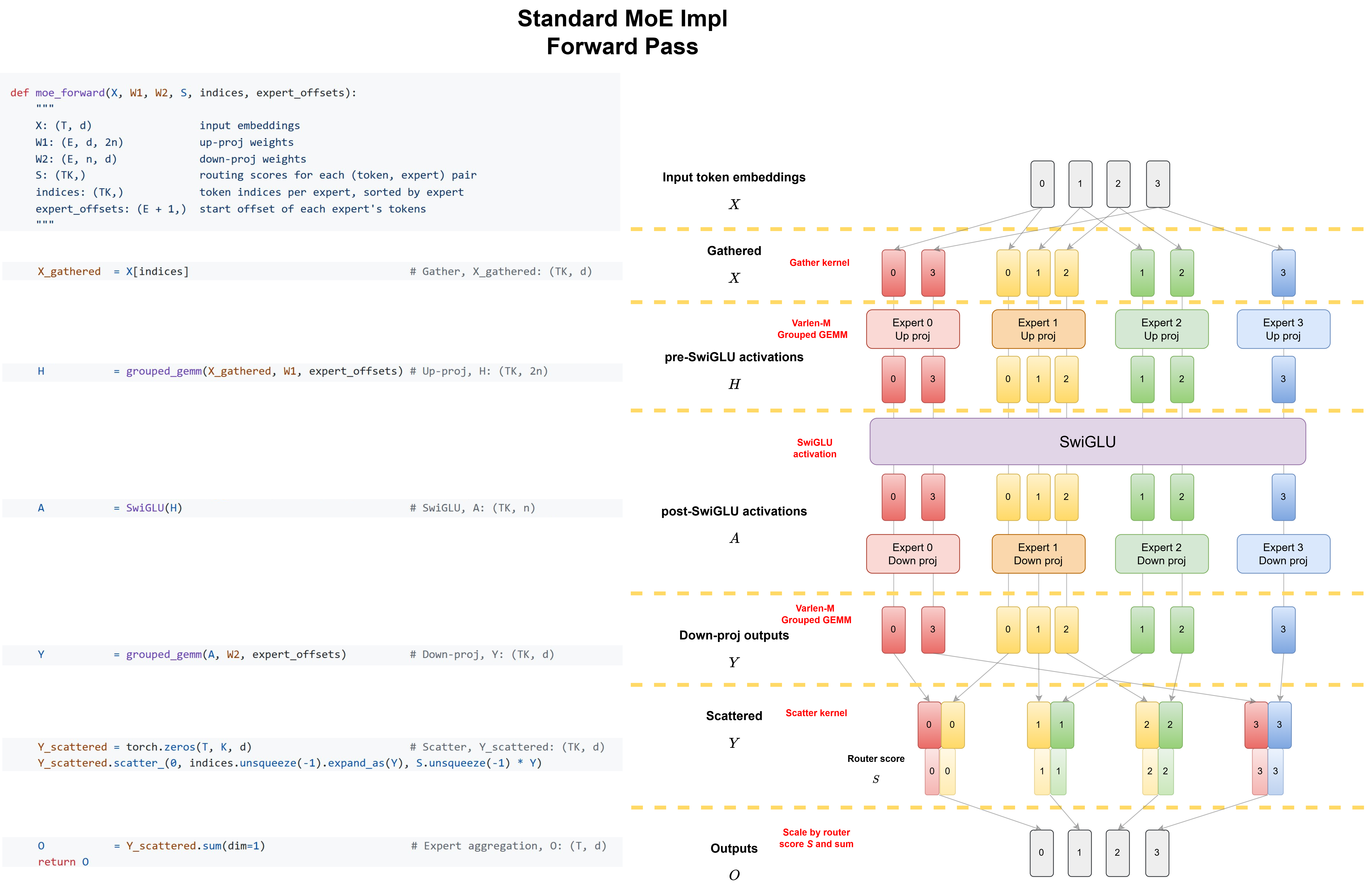
Figure: Visual workflow (left) with corresponding reference code (right) of standard MoE forward pass in PyTorch. Each yellow dashed line marks a kernel boundary. The standard implementation launches 6 separate kernels: gather, up-proj Grouped GEMM, SwiGLU, down-proj Grouped GEMM, scatter, and expert aggregation.
This can be simplified to the following workflow diagram:
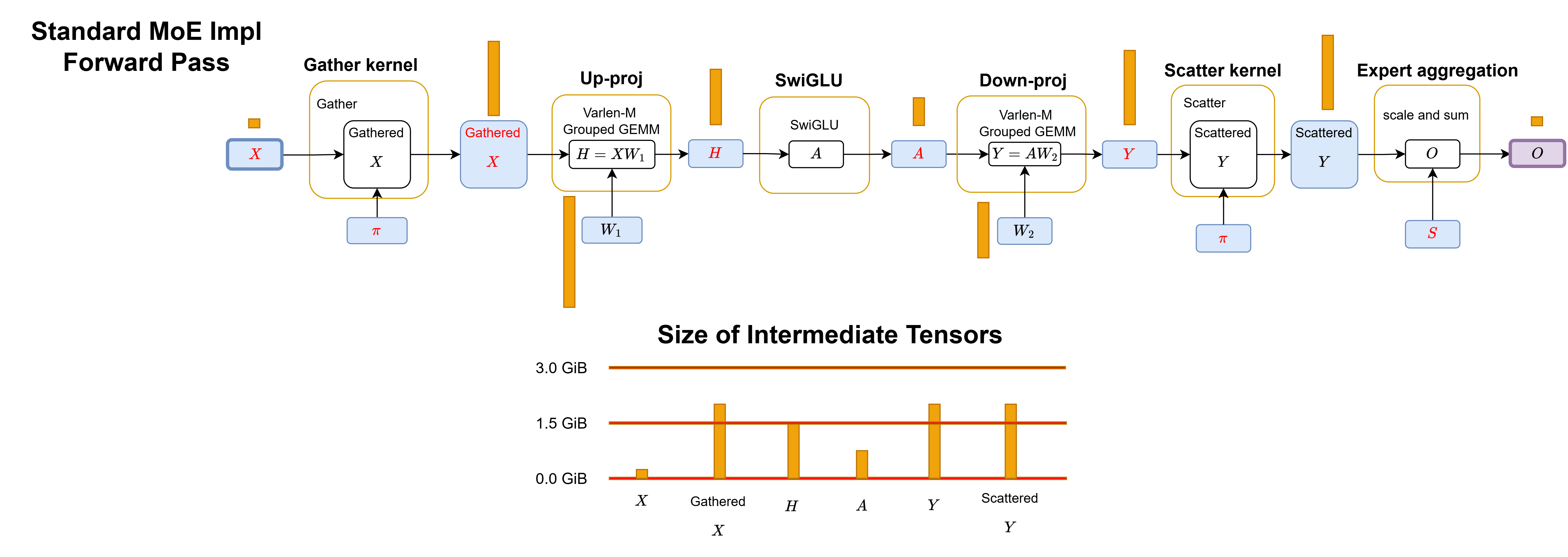
Figure: Workflow of standard MoE implementation forward pass. π is the binary mask that stores routing metadata. Yellow boxes are kernel boundaries. Blue boxes are variables in HBM. Red labels indicate the activations cached across the forward/backward. Purple boxes are the final outputs. The orange box beside each variable on global memory represents the tensor size in proportion for Qwen3-235B-A22B-Thinking-2507 MoE model with 32k tokens.
The workflow of backward activation gradient is simply a reverse operation with dSwiGLU as follows:
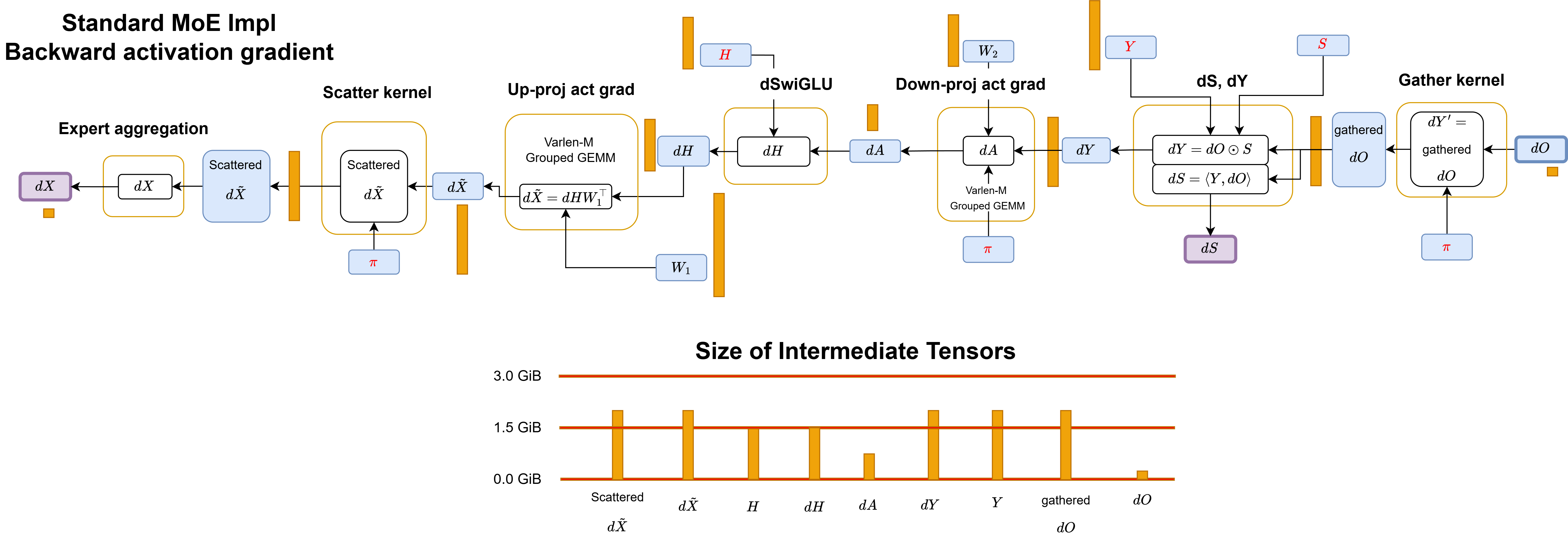
Figure: Workflow of standard MoE implementation backward activation gradient pass.
For weight gradient, we need to use varlen-K Grouped GEMM to reduce over token embeddings.
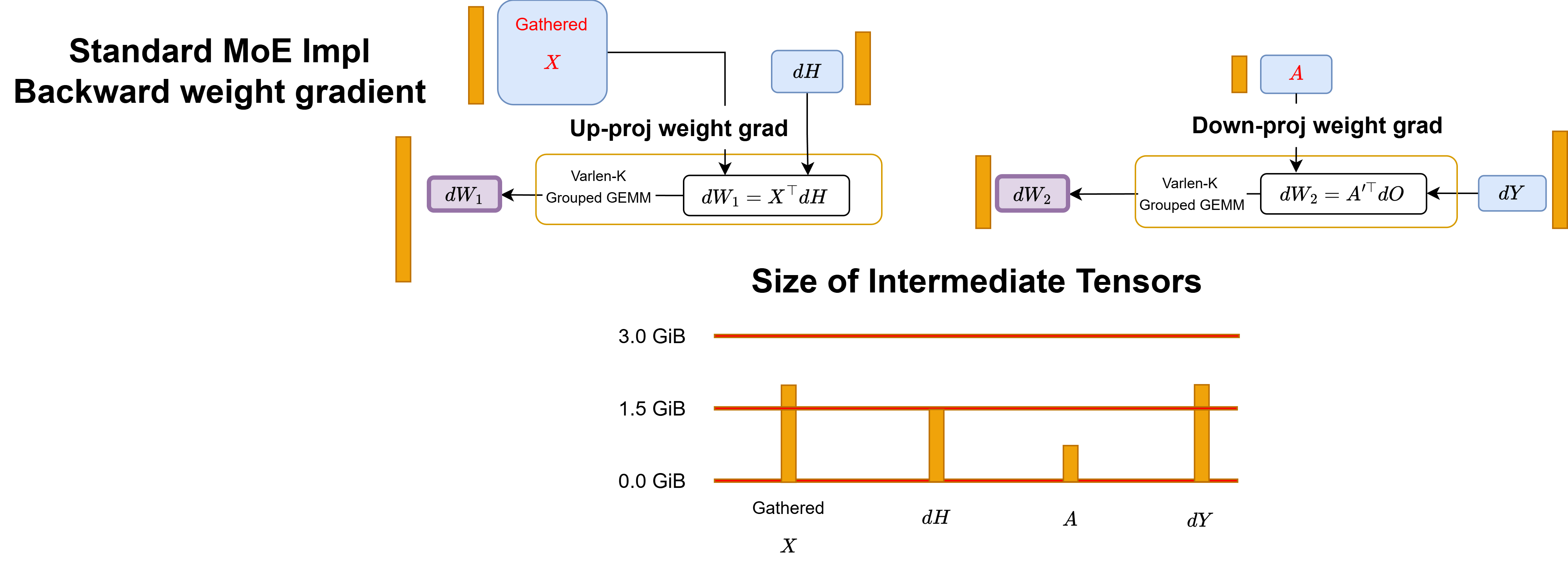
Figure: Workflow of standard MoE implementation backward weight gradient pass.
The standard implementation materializes every intermediate tensor in HBM between kernel launches. This creates two separate costs that both scale with expert granularity:
-
Activation memory: gathered \(X\), down-proj output \(Y\), and scattered \(Y\) must all be cached for the backward pass, each consuming \(2TKd\) bytes. As granularity increases, these \(O(TKd)\)-sized tensors grow linearly.
-
IO costs: every materialized intermediate is a round-trip to HBM. The backward pass is worse: it must additionally materialize \(dY\) and gathered \(dO\), both \(O(TKd)\)-sized. Since fine-grained MoE kernels operate in the memory-bound regime, these IO costs directly dominate runtime.
SonicMoE: the Algorithm and Kernel Decomposition
SonicMoE addresses both problems through a single algorithmic redesign: we circumvent the need to cache or materialize any variable with size \(O(TKd)\). This makes activation memory independent of expert granularity, and simultaneously eliminates multiple large HBM round-trips that dominate runtime.
In particular, SonicMoE avoids caching down-proj output \(Y\), scattered \(Y\), and gathered \(X\) which all have size \(T K d\). We also avoid writing \(dY\) and gathered \(dO\) to HBM:
-
Gathered \(X\) and \(dO\): we gather inputs at each kernel runtime and never cache the gathered results.
-
Scattered \(Y\): we fuse it with the aggregation operation where each token will gather and sum over activated expert results.
-
\(Y\) and \(dY\): we redesign the computational path that starts from \(dO\) and \(H\) to directly compute \(dS\) and \(dH\) during the backward pass without \(Y\) and \(dY\). Prior MoE kernels such as ScatterMoE and MoMoE must cache \(Y\) for this computation:
-
\(dH\): we apply gather fusion with \(dO\) (no need for \(dY\)) and dSwiGLU fusion with an extra load of \(H\).
-
\(dS\): we swap the contraction order. This is equivalent to placing \(S\) weighting before down-proj forward pass and using only \(A\) and \(dA'\) for computing \(dS\) instead of \(Y\) and \(dO\). We no longer need to cache \(Y\).
For an expert \(e\), denote the down-proj weights for expert \(e\) as \(W_{2,e}\in \mathbb{R}^{n\times d}\). The Grouped GEMM in down-proj activation gradient will compute \(dA' = dO_e W_2^\top\).
The standard path computes \(dS_{t,e} = \langle dO_t,\ Y_{e,t}\rangle\), which requires caching \(Y\). By substituting \(Y_e = A_e W_{2,e}\) and rearranging the contraction order:
\[dS_{t,e} = \langle dO_t,\ Y_{e,t}\rangle = \langle dO_t,\ A_e W_{2,e}\rangle = \langle dO_t W_{2,e}^\top,\ A_{e,t}\rangle = \langle dA_{e,t}',\ A_{e,t}\rangle\]Neither \(dA_{e,t}'\) nor \(A_{e,t}\) depends on \(dY\) or \(Y\).
-
Activation Memory Independent of Expert Granularity
SonicMoE’s forward pass. In the forward pass, SonicMoE only caches \(X\) and \(H\). The gathered results for \(X\) are never cached or materialized. The expert aggregation kernel fuses the scatter and summation together.
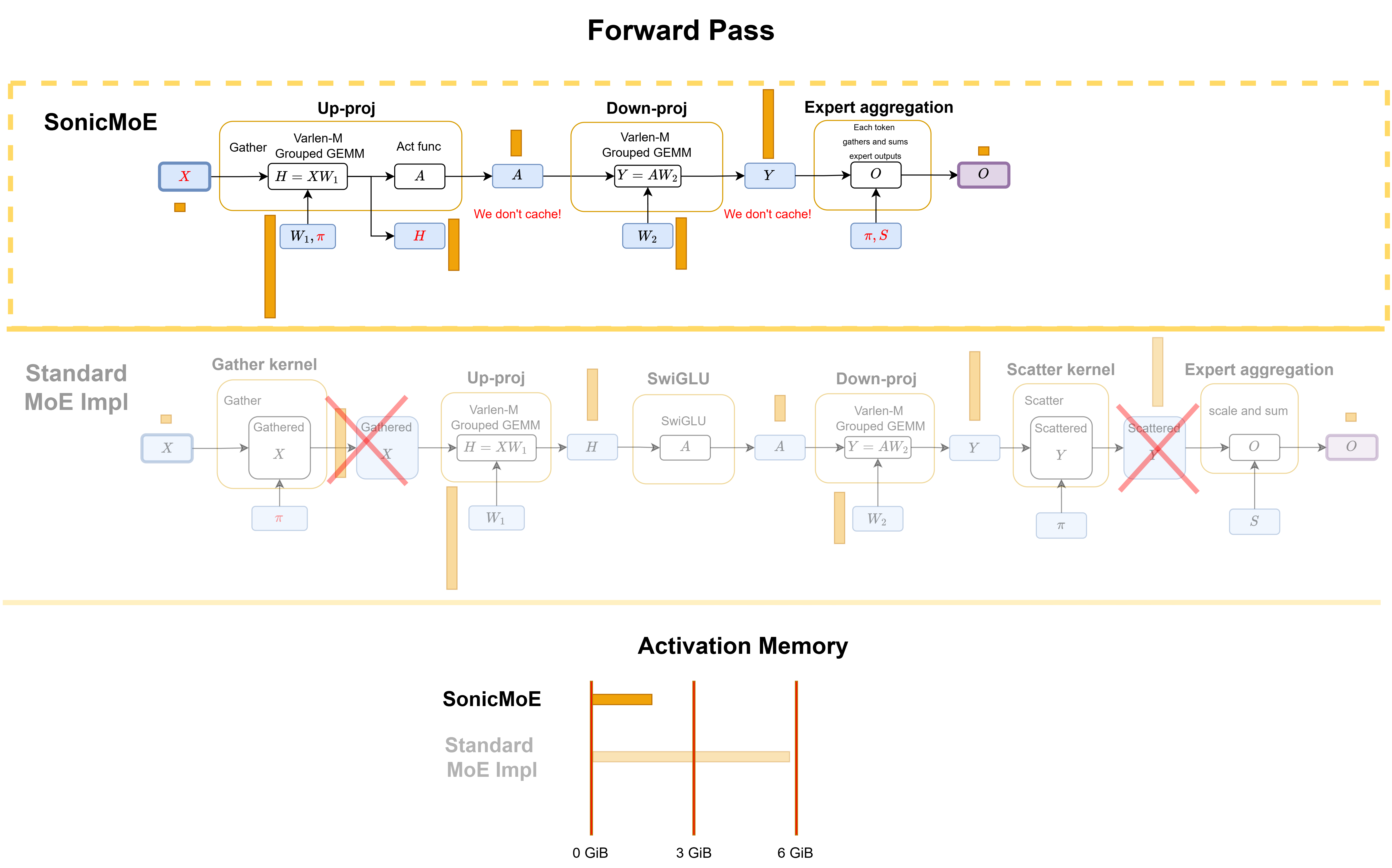
Figure: SonicMoE's forward computational workflow and comparison with a standard MoE implementation in PyTorch. We also compare the activation memory and IO costs for both methods.
The following figure gives a brief comparison on the activation memory breakdown. SonicMoE caches only inputs \(X\) and pre-SwiGLU activation \(H\) and does not need any GEMM recomputation.
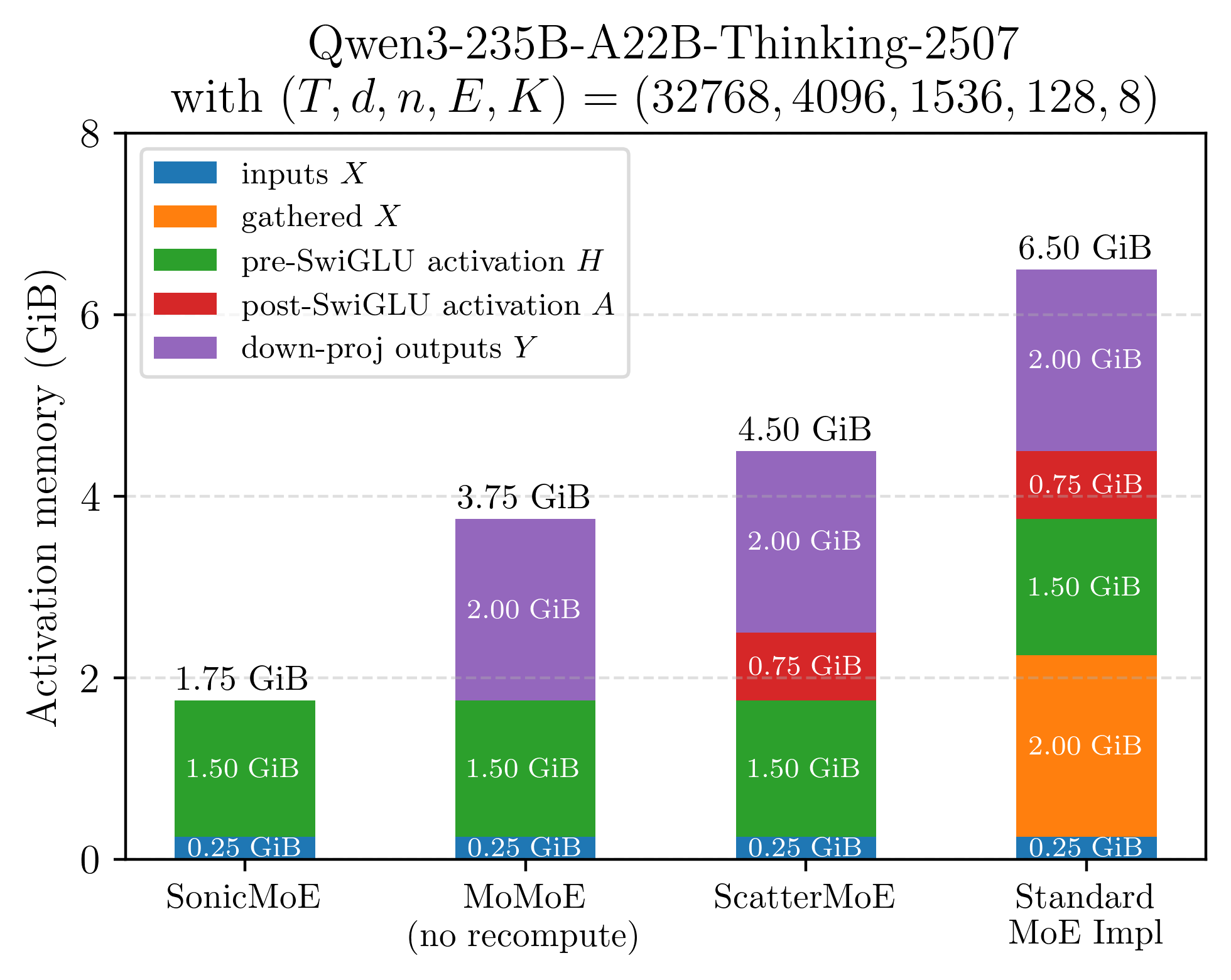
Figure: illustration of cached activation memory for a single layer of Qwen3-235B MoE model (microbatch=32k) when equipped with different training kernels.
SonicMoE can achieve the same activation memory efficiency as a dense model with the same activated number of parameters without extra training FLOPs.
IO Cost Reduction through Algorithmic Reordering
Each variable that is no longer cached is also one fewer read or write to HBM. The same redesign that eliminates \(O(TKd)\)-sized activations eliminates the corresponding HBM round-trips.
SonicMoE’s forward pass. We fuse the gather and SwiGLU activation in the up-projection. The scatter \(Y\) operation is fused with the expert aggregation.
SonicMoE’s backward pass.
-
Activation gradient: The down-proj activation grad \(dH\) kernel computes \(dH\), \(dS\), and \(A'\) (input for \(dW_2\)) simultaneously, none of which require caching \(Y\) or \(dY\). We similarly fuse dSwiGLU and the gather operation into the GEMM.
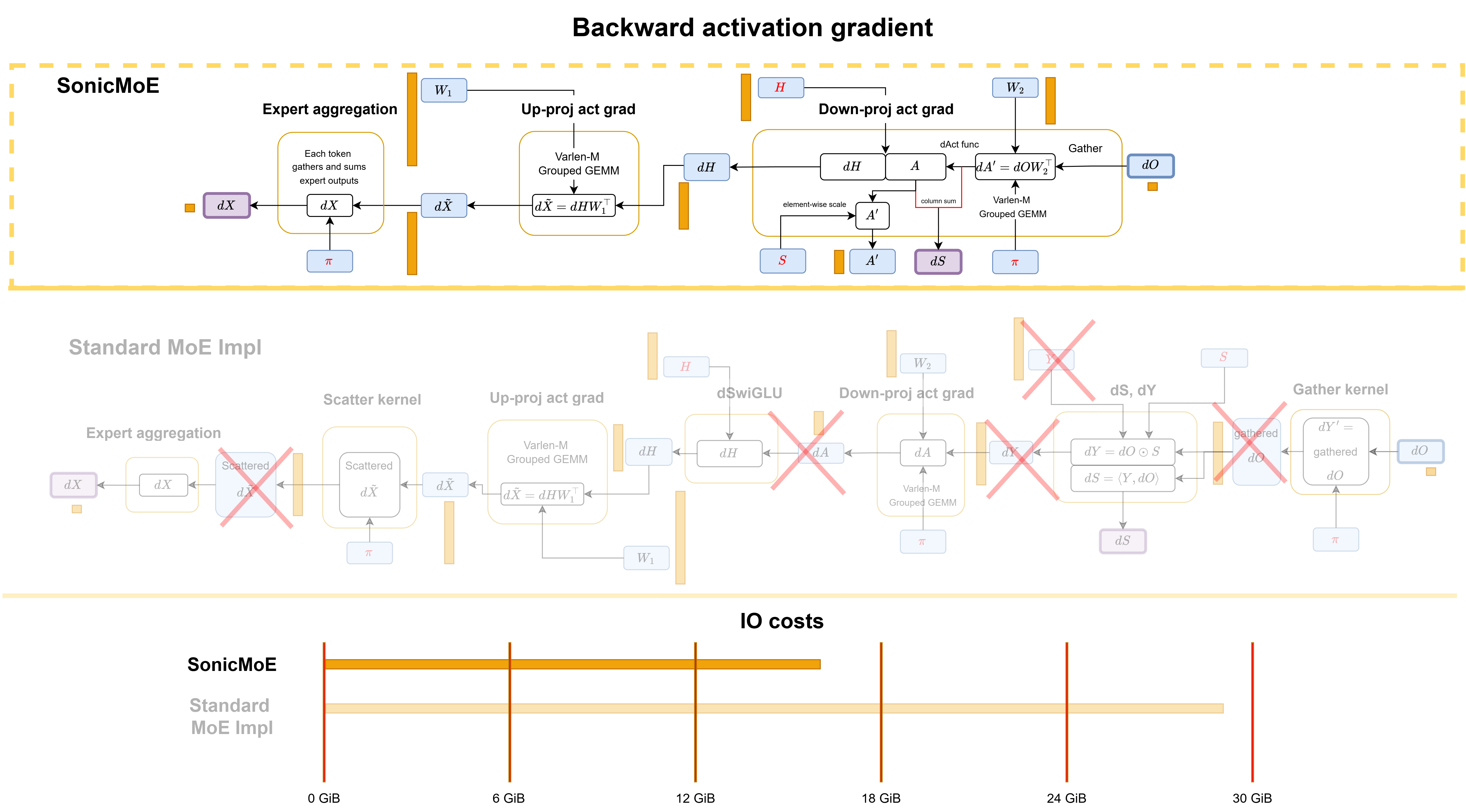
Figure: SonicMoE's backward computational workflow for activation gradient and comparison with a standard MoE implementation in PyTorch.
-
Weight gradient: The weight gradient kernels for \(dW_1\) and \(dW_2\) gather \(X\) and \(dO\) on the fly during execution. While their algorithmic IO costs match a standard MoE implementation, SonicMoE’s gather fusion reduces the hardware IO costs by exploiting L2 cache locality, which we will discuss later.
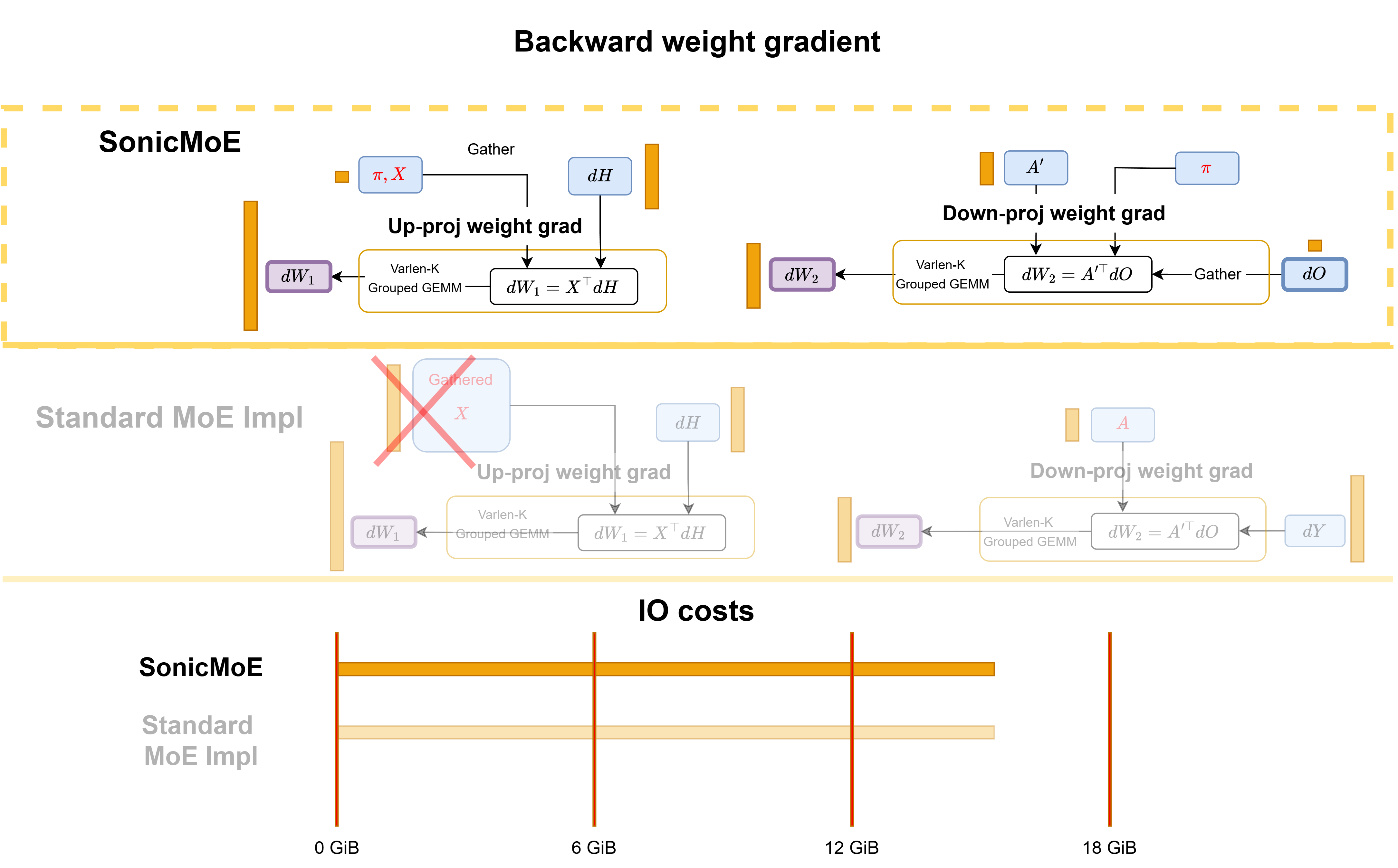
Figure: SonicMoE's backward computational workflow for weight gradient and comparison with a standard MoE implementation in PyTorch.
The net effect is a large reduction in IO costs even before any hardware-specific optimizations:
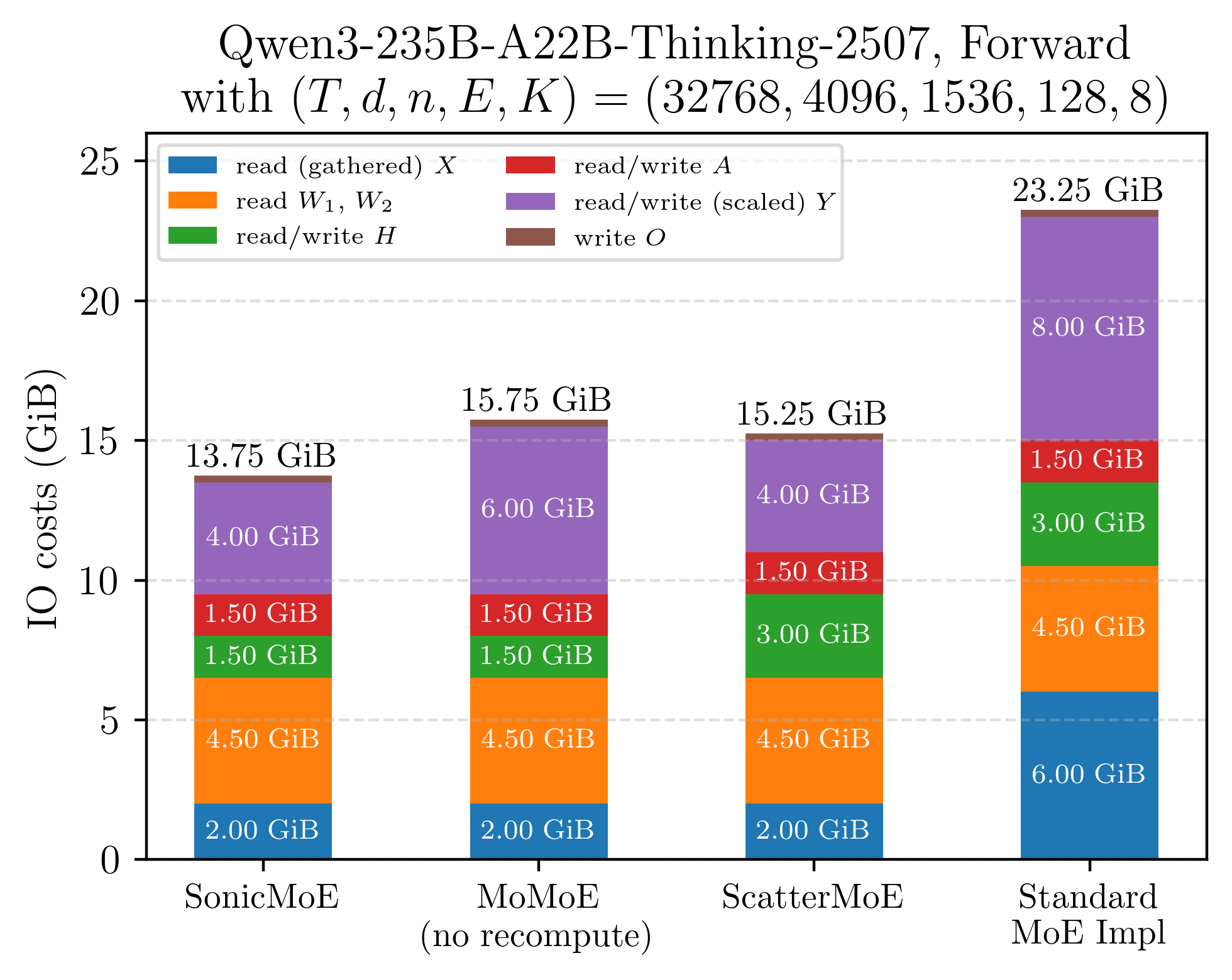
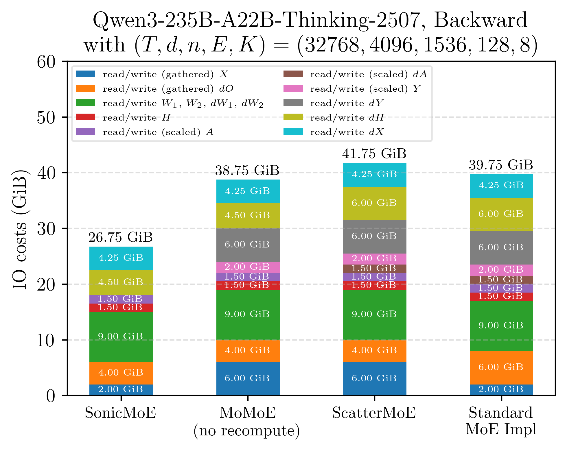
Figure: Illustration of IO costs for a single layer of Qwen3-235B MoE model (microbatch=32k) when equipped with different training kernels. SonicMoE's workflow circumvents the need to read or write multiple massive-sized tensors compared to existing MoE kernels.
Among these kernels, we want to give a special highlight to our backward down-proj activation gradient \(dH\) kernel as a combination of IO-aware and hardware-aware algorithmic design:
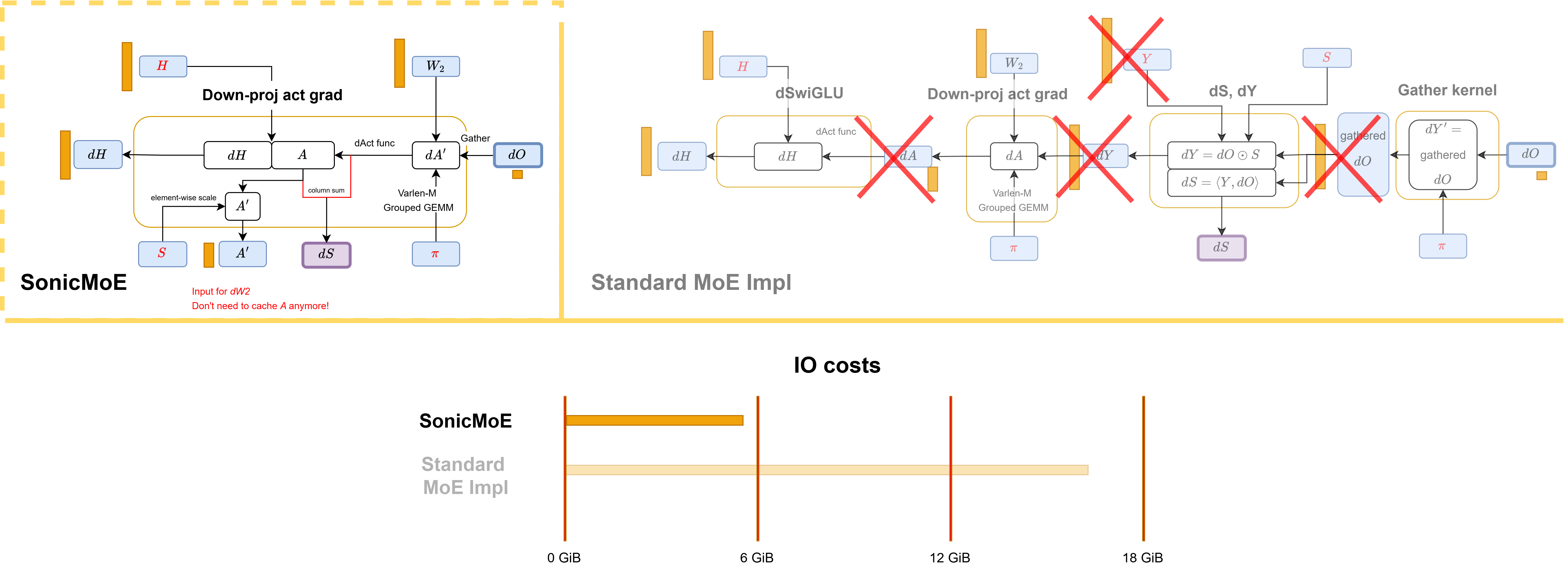
Figure: the semantics of SonicMoE's dH workflow diagram is equivalent to standard PyTorch MoE implementation for multiple kernels while SonicMoE substantially reduces the IO costs.
-
reduction of IO costs: we gather \(dO\), fuse the dSwiGLU call, and do not read or write \(Y\) and \(dY\).
-
hardware asynchrony features that further hide the remaining IO cost latency (will discuss later): the design of this \(dH\) kernel already reduces IO costs, and we further minimize the remaining impact of IO costs by leveraging the asynchrony features on modern NVIDIA GPUs.
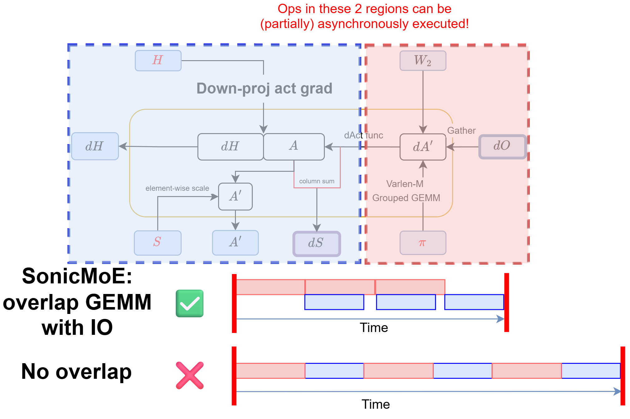
Figure: we can leverage recent NVIDIA hardware features to hide the IO latency in SonicMoE's dH kernel and greatly reduce the overall runtime.
A careful algorithmic design is sufficient to address the activation memory issue and partially the IO cost issue. We can further minimize the impact of IO costs by leveraging hardware asynchrony.
We want SonicMoE to achieve peak throughput on both Hopper and Blackwell GPUs, so we apply hardware-aware optimizations to all Grouped GEMM kernels in SonicMoE. However, modern NVIDIA GPU architectures often differ substantially in their execution models. In response, we build a unified and modular software abstraction that expresses all grouped gemm kernels while localizing all architecture-specific optimizations to a small number of overrides. The rest of this post describes that abstraction and how it is realized on each architecture.
2. the Software Abstraction of QuACK that Empowers SonicMoE
SonicMoE already supports NVIDIA Hopper (SM90), Blackwell GPUs (SM100), and the support for Blackwell GeForce (SM120) GPUs is on the way. When we first considered porting the Hopper kernels to Blackwell, the straightforward path was to rewrite 6 Grouped GEMM kernels from scratch. We chose instead to factor out the shared structure, and this decision proved highly productive later.
Every Grouped GEMM kernel is an instance of the same underlying structure: a producer-consumer GEMM mainloop that overlaps data movement with tensor core computation, followed by a parameterized epilogue that applies fusion logic directly to the accumulator before any data reaches HBM.
This shared structure of GEMM mainloop with customizable epilogue would make SonicMoE’s implementation modular, extendable to new hardware while still maintaining peak performance.
We also unify the API and encapsulate other architecture-specific changes. SonicMoE’s GEMM kernels are built on top of QuACK, our in-house CuTeDSL library that draws heavily from CUTLASS and the CuTeDSL official examples. CUTLASS defines a clean layered programming model for GPU kernels: a mainloop that tiles the matrix multiplication across the parallel workers (Streaming Processors), and an epilogue that post-processes the results before writing them back to memory. QuACK adopts this layered programming model and extends it with modular components (tile schedulers, customizable epilogue, etc.).
Below, we examine the design of QuACK GEMM and how it helps SonicMoE achieve peak throughput amid high IO costs.
Tiled GEMM kernel on NVIDIA GPUs
A General Matrix Multiplication (GEMM) kernel on NVIDIA GPUs repeatedly fetches tiles of input data \(A,B\) (\(A\) is usually the activations while \(B\) is the weights), and we accumulate the tiled MMA (matrix multiply-accumulate) results into a zero-initialized buffer \(C\) (often the output activations).
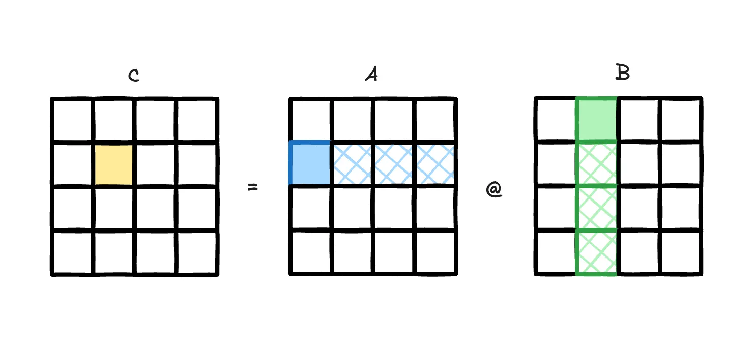
Figure: illustration of GEMM tiled accumulation [2]
Repeated 3-phase Accumulation for Each Output Tile
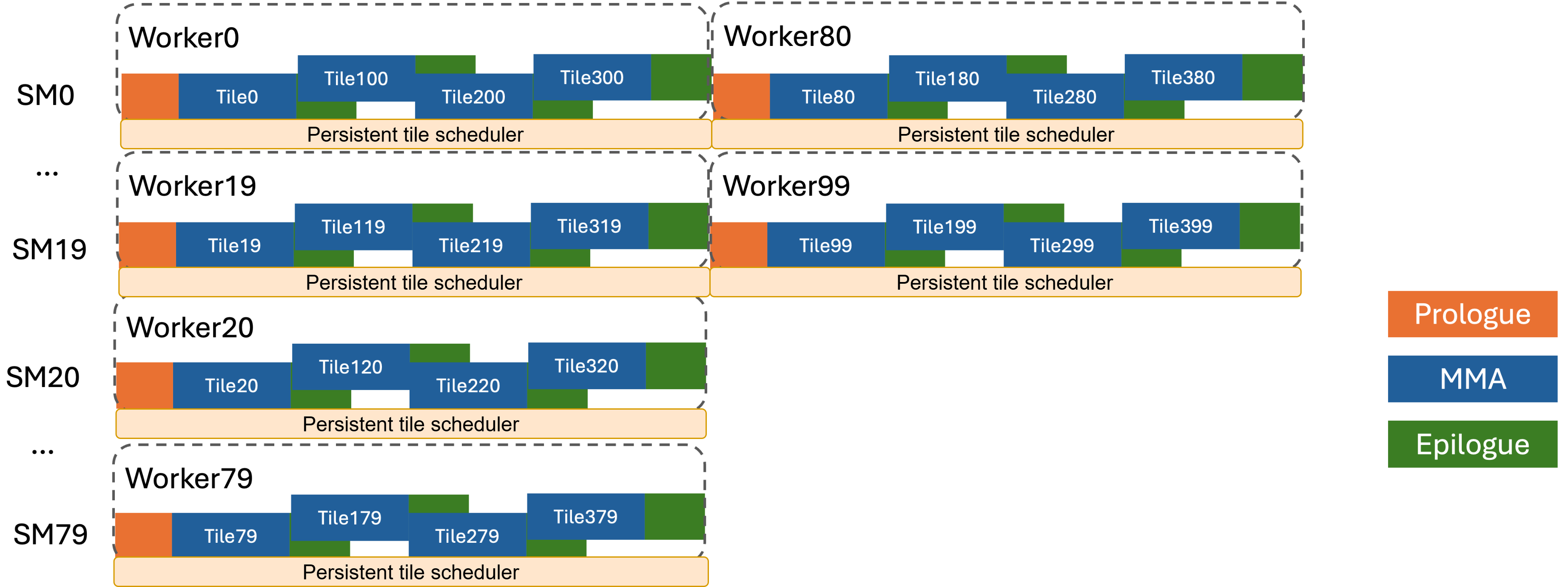
Figure: each Streaming Processor (SM) on GPUs will perform tiled MMA in 3 phases until no tiles left. Usually there will be a persistent tile scheduler that schedules which tile each SM will receive. Adapted from [3].
For every output tile, the accumulation process is formulated into three phases:
-
Prologue (by producer): the load warp(s) load the inputs to fill SMEM buffers with tiles of A and B.
-
Mainloop (input loading by producer, MMA by consumer): the MMA warp/warpgroup consumes filled shared memory (SMEM) buffers, executes the MMA instruction, and accumulates into an output buffer. On Hopper this result buffer lives in registers (WGMMA). On Blackwell the result lives in TMEM (UMMA).
-
Epilogue (by consumer): the consumer warpgroup (Hopper) or the dedicated epilogue warps (Blackwell) apply any fused post-processing to the accumulated results, and write back to GMEM (global memory, often the HBM).
This three-stage structure is the same for all 6 Grouped GEMM kernels in MoE. What changes between kernels is exclusively the following:
- How the producer loads the data when we have contiguous or gathered inputs
- What the epilogue consumer does to the accumulator before writing it to GMEM
Point (1) is the gather fusion described in Section 4. Point (2) is where all MoE-specific fusion logic lives, and it is the core of QuACK’s customizable epilogue abstraction.
Tile Scheduling: Decide which Output Tile to Process by Each CTA
A persistent tile scheduler will give a unique tile coordinate to each CTA (thread block, usually 1 per SM) until all tiles are consumed. Multiple modes of tile schedulers are supported and selected automatically based on architecture and kernel configuration:
-
Static (SM90 default): fixed linear tile-to-CTA assignment.
-
Cluster Launch Control (CLC) (SM100 default): hardware-assisted cluster-level dynamic scheduling via the Blackwell-specific
clusterlaunchcontrol.try_cancelPTX instruction. The hardware manages the work queue. We will describe CLC in detail in Section 3.
Customizable Epilogue
The base GEMM class implements the epilogue as a fixed loop skeleton. For each sub-tile of the output:
- Load the accumulator fragment into a register tensor
- Call
epi_visit_subtileto execute customized epilogue ops. - Write epilogue results to shared memory and finally to global memory
The epi_visit_subtile method is a no-op in the base class. Subclasses override it to inject arbitrary per-element fusion logic. This single method is the injection point for every activation function, every backward pass computation, every scaling operation, and every reduction in the entire SonicMoE codebase.
Each epilogue mixin (e.g., GemmGatedMixin for SwiGLU, GemmDGatedMixin for the \(dH\) backward) is paired with an architecture-specific base class: GemmGatedSm90 / GemmGatedSm100, GemmDGatedSm90 / GemmDGatedSm100, etc. The architecture-specific suffix controls only the warp layout, accumulator movement (registers vs. tensor memory), and hardware resource management. The epilogue fusion logic in epi_visit_subtile is shared across architectures. For example, the heaviest kernel in SonicMoE is just a GemmDGatedMixin with additional arguments, implemented in 88 lines:
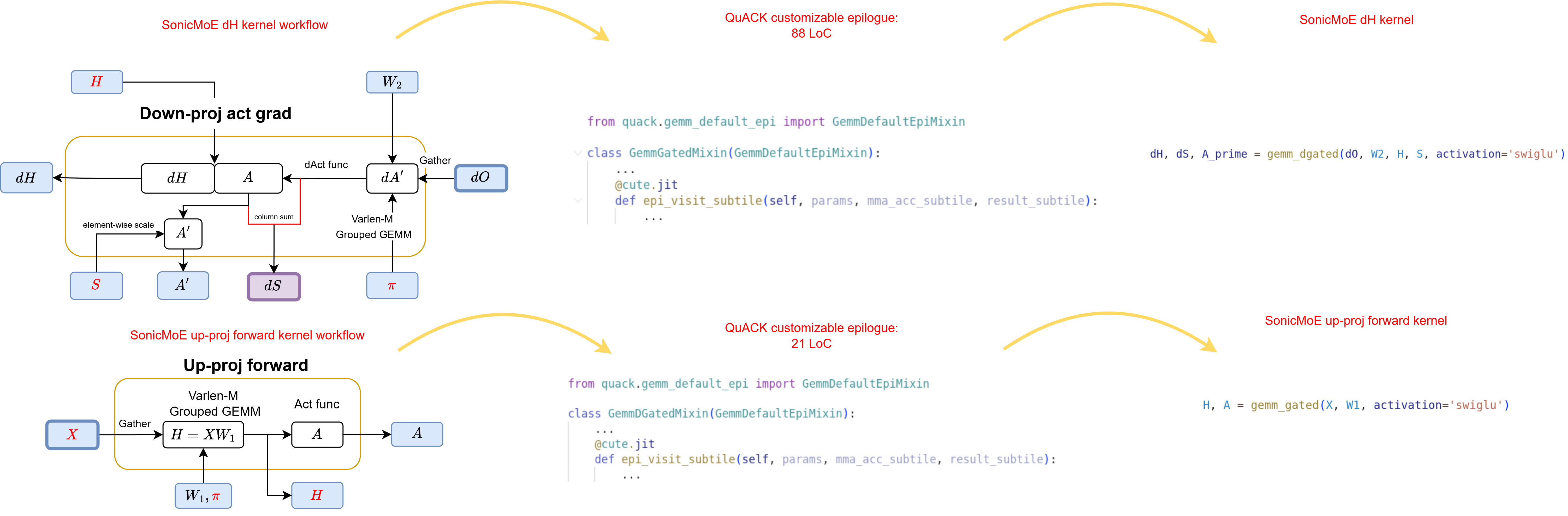
Figure: Two SonicMoE kernels implemented with QuACK. Left: the kernel workflow diagram. Center: the QuACK epilogue mixin class where each kernel overrides `epi_visit_subtile` (88 LoC for dH, 21 LoC for up-proj forward). Right: SonicMoE's simplified kernel launch call.
In total, this software abstraction on QuACK delivers three properties we prioritize:
-
Adaptability to new model architecture or algorithms: future developers need only modify how epilogue works to provide a fast kernel implementation for other model architectures or algorithms, not only MoE.
- For example, Gram Newton-Schulz is also built on top of symmetric gemm on QuACK, with the quote from its blogpost:
Using these abstractions, we are able to implement the symmetric GEMM kernel for both Hopper and Blackwell in just 160 lines, while achieving SOTA performance.
- We also only write ~200 LoC to implement SonicMoE on top of QuACK Grouped GEMM which works automatically on both Hopper and Blackwell GPUs.
- For example, Gram Newton-Schulz is also built on top of symmetric gemm on QuACK, with the quote from its blogpost:
-
Fast extensibility to new hardware (features): a unified API from top to bottom across different hardware architectures.
We can change our base GEMM implementation and the existing kernels should work on the new hardware, which enables quick research development:
-
We develop TMA gather4 for Grouped GEMM on Blackwell GPUs by simply modifying copy atoms and SMEM layouts with ~100 LoC changes. We do not change anything on the MMA warps.
-
We extend to SM120 (Blackwell GeForce GPUs such as 5090) by simply adding a base GEMM class with ~500 LoC changes. We do not change anything on the customizable epilogue and GEMM interface.
-
-
Codebase maintainability: the new modular design reduces the cost of future maintenance and makes the codebase accessible to new contributors.
- Our prior Hopper Grouped GEMM integrated 3-phase GEMM programming model and all possible fusions together, with more than 3k lines of code. This complexity placed a significant burden on maintainers and made adding new features error-prone.
In the next section, we will describe how SonicMoE benefits from new Blackwell features.
3. Underneath the Abstraction: Hardware Features that Empower the IO Overlap
The software abstraction described in the previous section was designed so that all architecture-specific behavior is confined to a small number of localized overrides. This section describes what Blackwell provides at the hardware level, and why each new feature maps cleanly onto one of those overrides.
GEMM programming model
On Hopper, MMA is usually performed via a warpgroup-level instruction WGMMA (wgmma.mma_async). It requires 128 threads (4 contiguous warps) to issue and manage: all threads in the warpgroup participate in tracking the accumulator state, and the accumulator result is distributed across the register files of those 128 threads. We often have 2 consumer warpgroups, and we can either let them cooperatively issue 2 WGMMA instructions, or we can overlap the IO of 1 warpgroup with the GEMM of another warpgroup. In this case, we can let 1 consumer warpgroup do MMA while the other consumer warpgroup does the epilogue, and they switch roles once each finishes. This is called “Ping-Pong warpgroup scheduling”, often particularly useful to maintain high Tensor Core throughput with heavy epilogue.
For example, the down-proj forward kernel’s epilogue has heavy HBM store IO relative to the mainloop. In the \(dH\) kernel’s epilogue, we need to load \(H\) and execute multiple activation and reduction operations to compute and store \(dH\), \(dS\), and \(A'\) as inputs for \(dW_2\).
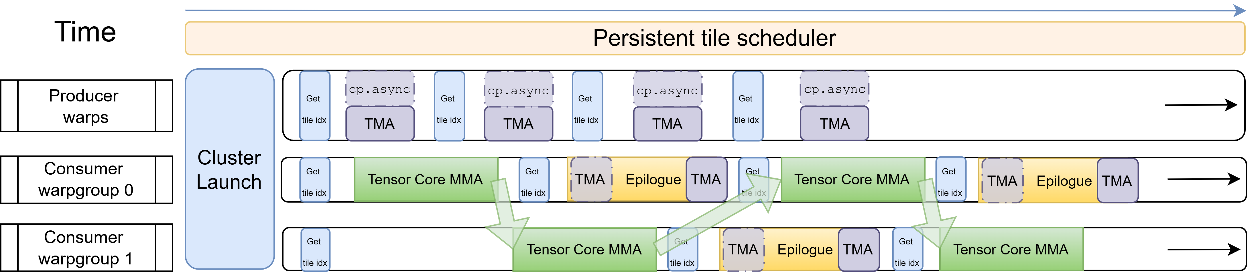
Figure: Hopper Ping-Pong: two consumer warpgroups alternate between MMA and epilogue: while one runs Tensor Core MMA, the other runs the epilogue (TMA store + any async load). Green arrows show the signal from one warpgroup that the other can proceed.
On Blackwell, new UMMA (tcgen05.mma) instruction breaks this coupling entirely. UMMA is single-threaded asynchronous: one thread in the warp issues it, and execution proceeds asynchronously without occupying any other threads or registers. The accumulator result is written directly into Tensor Memory (TMEM) — a new dedicated 256 KB on-chip memory per SM that is wired into the tensor cores and completely separate from the register file.
TMEM is organized as 128 rows × 512 columns of 32-bit cells, for a total of 256 KB per SM. The 512-column structure can hold two independent accumulator stages of 256 columns each. This is the hardware basis for Blackwell’s MMA/epilogue overlap as shown below.
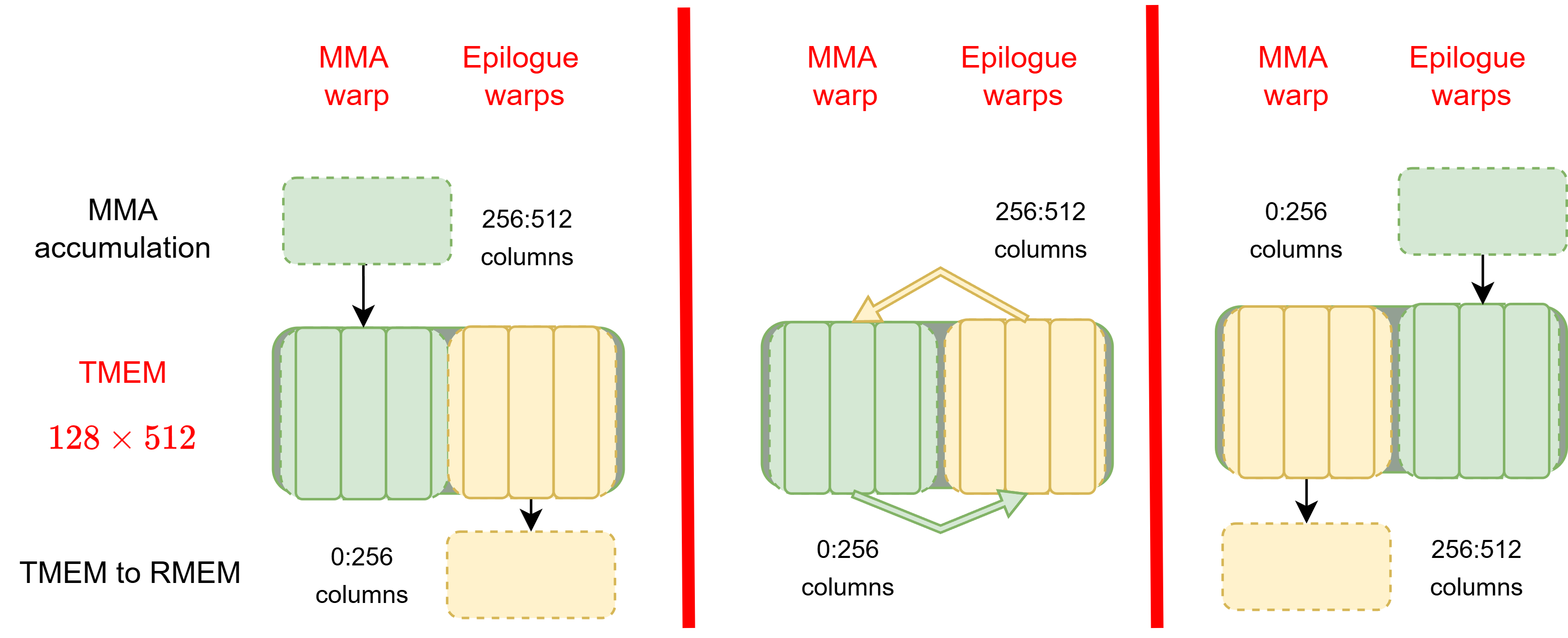
Figure: TMEM column ownership transfer between MMA warp and epilogue warps. This technique is often referred to as "double-buffering".
While the MMA warp accumulates into one 256-column stage, the epilogue warps are simultaneously draining the other stage via tcgen05.ld (the TMEM-to-register copy instruction) and performing epilogue ops afterwards. When the epilogue warps finish and signal via the accumulator pipeline, the MMA warp acquires the next stage and begins filling it. The stages alternate every tile. This is Ping-Pong in spirit as it overlaps MMA with epilogue IO.
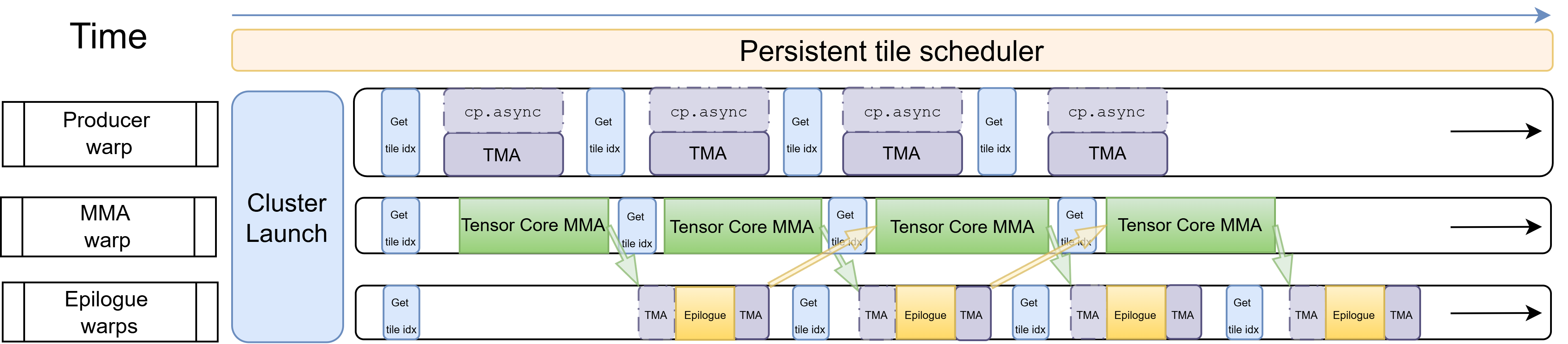
Figure: Blackwell warp-specialized pipeline: one producer warp (top), one MMA warp (middle), multiple epilogue warps (bottom) running concurrently. Green arrows show the ready signal of TMEM stage from the MMA to epilogue warp. Yellow arrows show the release signal of TMEM stage from the epilogue to MMA warp.
2CTA MMA
A second major Blackwell feature is the cta_group::2 variant of UMMA. When this mode is enabled, a pair of CTAs in the same cluster cooperatively execute a single MMA instruction. The tile M dimension doubles: where a single-CTA UMMA supports up to \(M_\mathrm{tile}=128\), a 2CTA UMMA supports up to \(M_\mathrm{tile}=256\).
For a tile of shape \(M_\mathrm{tile} \times N_\mathrm{tile} \times K_\mathrm{tile}\), the number of FLOPs is \(2 M_\mathrm{tile} N_\mathrm{tile} K_\mathrm{tile}\) and the number of bytes loaded from SMEM is \(2(M_\mathrm{tile} K_\mathrm{tile} + N_\mathrm{tile} K_\mathrm{tile})\) for A and B. For fixed \(N_\mathrm{tile}\) and \(K_\mathrm{tile}\), doubling \(M_\mathrm{tile}\) doubles the FLOPs but only adds \(2M_\mathrm{tile} K_\mathrm{tile}\) bytes of A data — the B tile of shape \(N_\mathrm{tile} \times K_\mathrm{tile}\) is shared across the pair, so each CTA loads only half the B data it would need for two independent 1CTA tiles. This is the key benefit: the B tile is multicasted via TMA across the CTA pair, halving B-side SMEM traffic per output element.
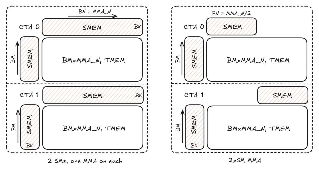
Figure: independent 1CTA MMA (left) vs. 2CTA MMA, referred to as 2xSM MMA in the figure (right). Left: two separate CTAs each load a full B tile and hold a full accumulator in TMEM. Right: in 2CTA MMA, B tile is halved and shared. Each CTA holds the full accumulator on TMEM but loads only half the B data. [4]
Native Dynamic Persistent Tile Scheduler
A persistent tile scheduler is essential for MoE kernels because it allows one CTA to begin loading the next tile while the current tile’s epilogue is still in progress, keeping both the producer and consumer pipelines continuously occupied.
On Hopper, we often have a fixed, static linear pre-assignment of tiles to CTAs (we call it “static tile scheduler”). This induces zero synchronization overhead, but it is susceptible to workload imbalance when expert token counts vary. Implementing a dynamic persistent tile scheduler aware of each SM’s progress requires a global semaphore counter in GMEM and atomic traffic. The advantage of dynamic persistent over static persistent is often not obvious or decisive.
Blackwell introduces Cluster Launch Control (CLC): a hardware instruction clusterlaunchcontrol.try_cancel that lets a running cluster query the hardware for its next tile coordinate without touching GMEM atomics. The hardware manages the work queue, operates at cluster granularity, and returns either a tile coordinate or a decline signal when all tiles are processed. The query to the hardware has minimal overhead and the response is broadcast to the whole cluster at once, eliminating per-CTA atomic traffic entirely.
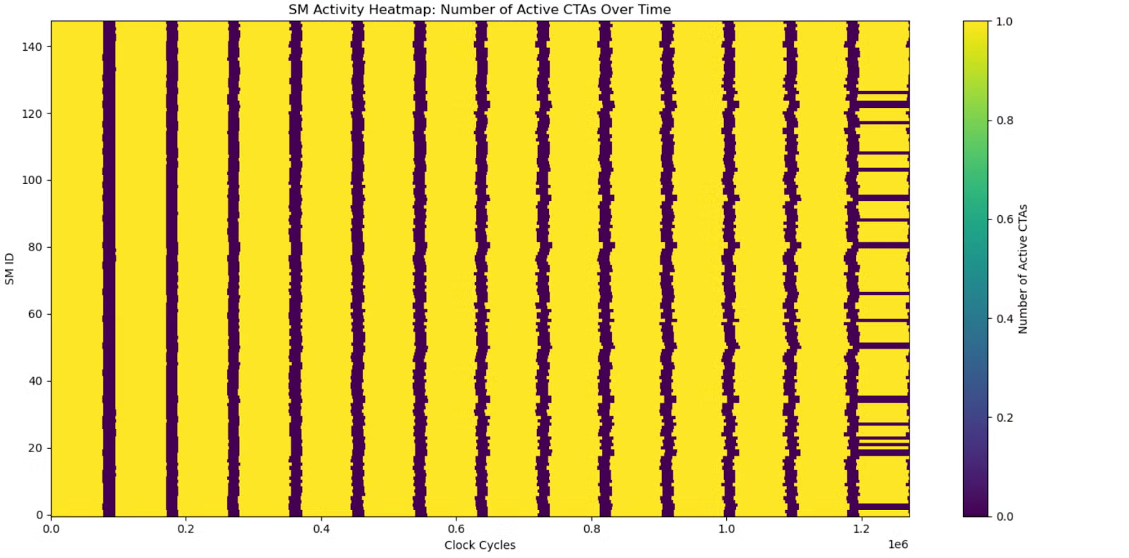
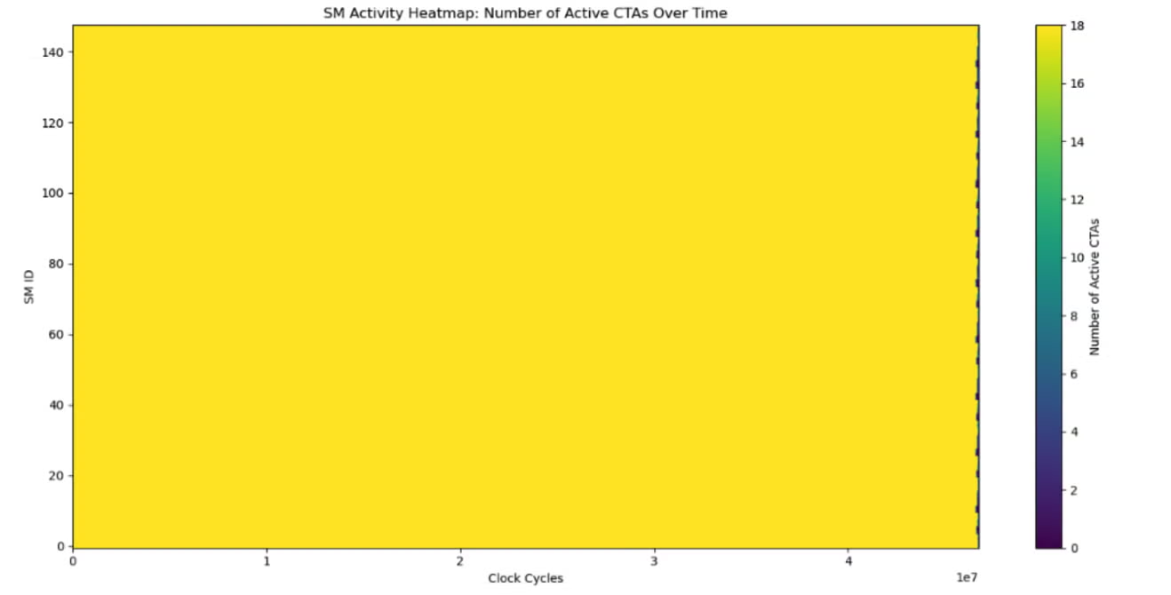
Figure: SM heatmap without persistent tile scheduler (left) and with CLC tile scheduler (right) [5]. The CLC tile scheduler can help all SMs stay active throughout the kernel runtime.
The CLC tile scheduler and extensive use of 2CTA MMA in varlen-M Grouped GEMM already help SonicMoE to achieve higher throughput (~10\%) than both DeepGEMM sm100_m_grouped_bf16_gemm_contiguous and triton official example. We compare SonicMoE’s implementation with the DeepGEMM and triton official example in the appendix.
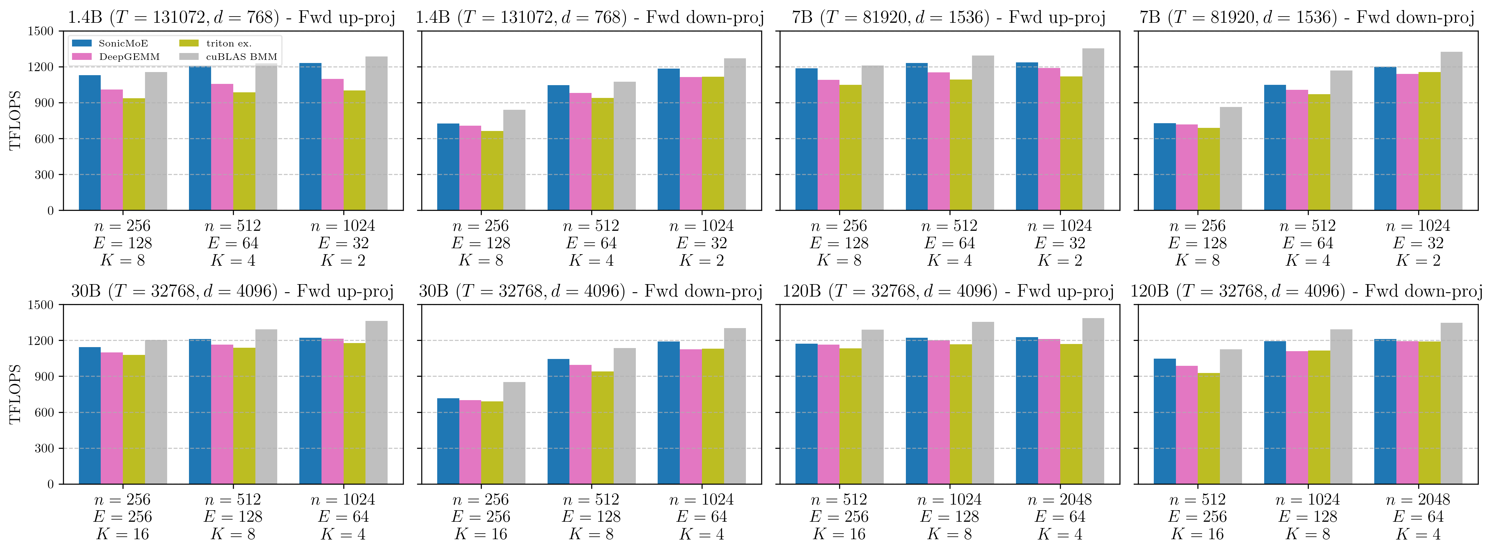
Figure: Varlen-M Grouped GEMM with contiguously-packed inputs on B300 GPUs. Detailed descriptions of other baselines can be found in the caption of Figure 18 of our arXiv paper.
4. Reducing the Impact of IO Costs
The hardware features described in Section 3 provide the infrastructure for high throughput. But for fine-grained MoE, the dominant cost is not raw MMA throughput: it is the IO overhead of gathering tokens from arbitrary positions and of executing heavy epilogue computations without stalling the tensor cores. This section describes the three fusion principles that address these costs, and how each one is adapted for Blackwell.
Gather Fusion
Multiple varlen-M GEMMs in SonicMoE read tokens from arbitrary positions in the input tensor where the routing decision determines which rows of \(X\) (or \(dO\)) belong to each expert. SonicMoE fuses the gather directly into the GMEM-to-SMEM load. On Blackwell GPUs, SonicMoE will dispatch to gather with either cp.async or TMA gather4 (cp.async.bulk.tensor.2d.shared::cta.global.tile::gather4 gathers 4 rows each time), whichever is faster at autotuning stage.
-
cp.asyncgather fusion with 2CTA MMA. When 2CTA MMA is combined with cp.async gather fusion, a synchronization challenge arises: cp.async can only signal completion within its own CTA, but the leader CTA’s MMA needs both CTAs’ data ready. We resolve this with a dedicated relay warp in CTA 1 (non-leader) that forwards the completion signal to CTA 0 (leader) via a cluster-scope barrier.
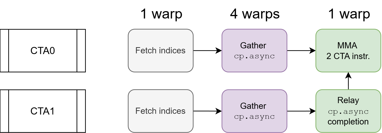
Figure: 2CTA MMA relay mechanism. CTA 0 (top) as the leader CTA: 1 warp fetches indices, 4 warps issue `cp.async` gathers, 1 warp issues the 2CTA MMA instruction after waiting at its barrier. CTA 1 (bottom): 1 warp fetches indices, 4 warps issue `cp.async` gathers, 1 relay warp waits for the `cp.async` completion and then arrives at CTA 0's barrier.
We then compare the speed of SonicMoE’s gather fusion against other MoE kernels’ GEMM with a separate gather kernel or with gather fusion. SonicMoE’s gather fusion is only 1.4% slower on the M dimension and 0.5% faster on the K dimension relative to contiguous inputs. Therefore, SonicMoE consistently achieves higher TFLOPS than ScatterMoE, MoMoE, and the triton official example even with gather fusion.
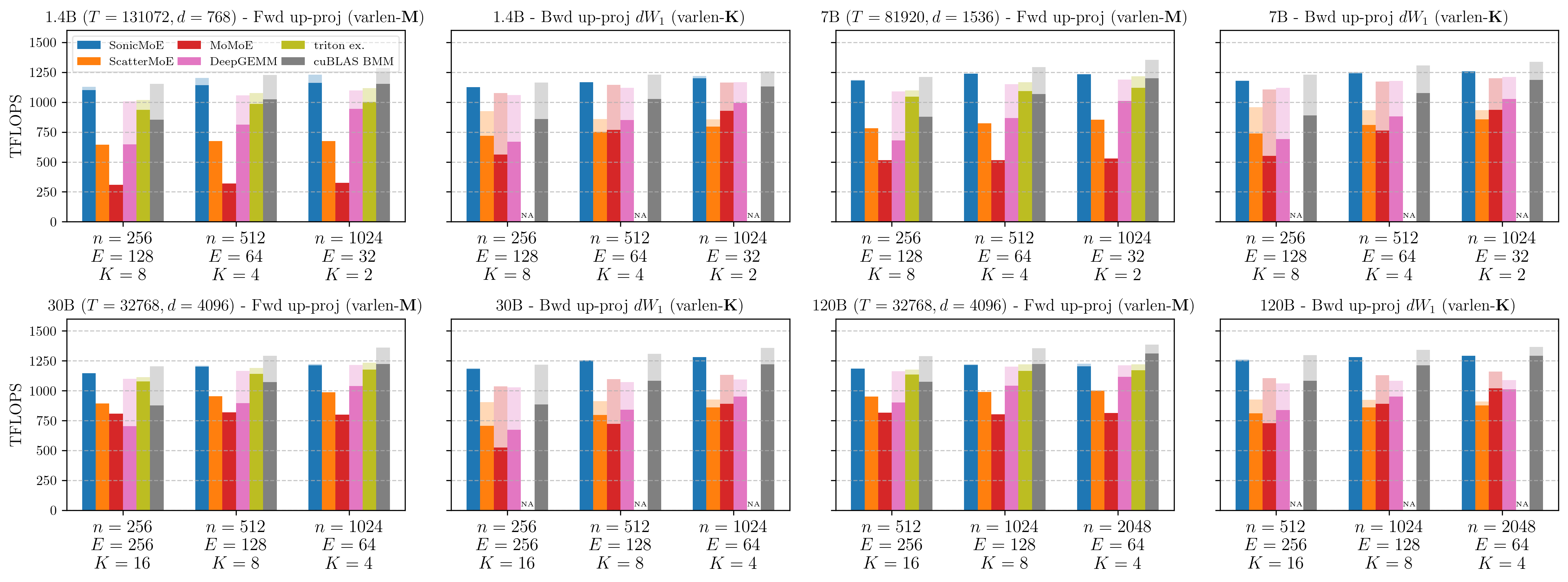
Figure: Forward pass up-proj (gather on M dim) and backward dW1 kernel (gather on K dim) kernel on B300 GPUs. SonicMoE supports both inputs gathered from different positions (opaque bars) and contiguously-packed inputs (transparent bars). Detailed descriptions of other baselines can be found in the caption of Figure 19 of our arXiv paper.
Gather Fusion Reduces Hardware IO costs via L2 Cache Locality
The L2 cache sits between HBM and SMEM in the GPU memory hierarchy and is shared across all SMs. All traffic between SMs and HBM flows through L2: when an SM requests data that is already cached, the request is served at L2 bandwidth (~20 TB/s [7]) without touching HBM. When the request misses, the data is fetched from HBM (7.7 TB/s) and inserted into L2 for future reuse.
A common alternative to gather fusion is to run a separate gather kernel that pre-arranges the inputs into a contiguous buffer before the Grouped GEMM. Although both approaches have identical algorithmic IO costs (assuming no TMA multicast along the N dimension), gather fusion reduces the actual HBM load traffic through better L2 cache utilization.
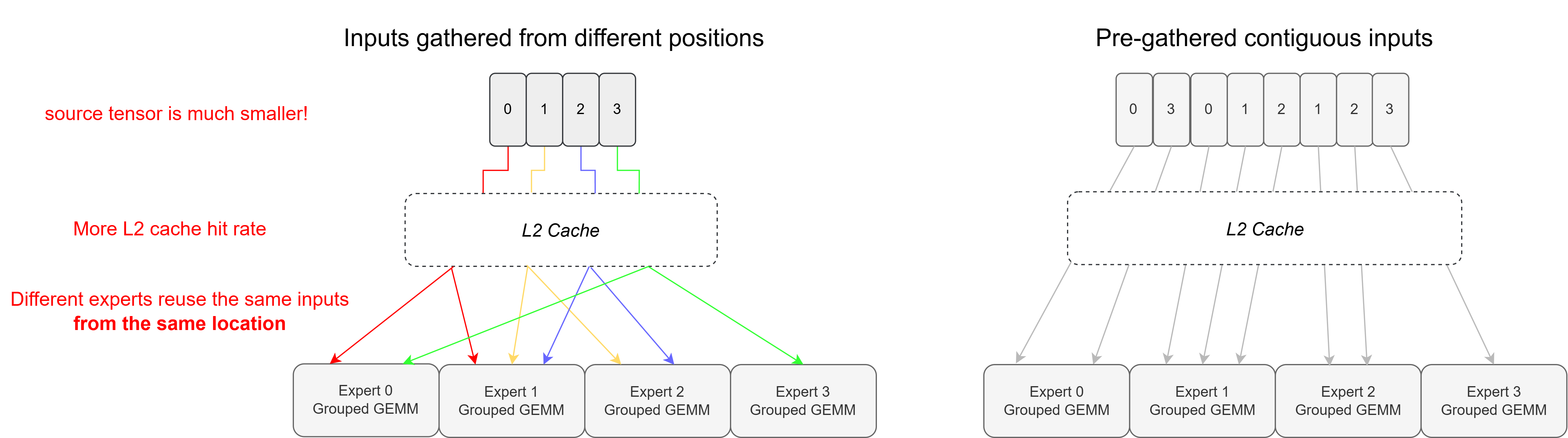
Figure: Gather fusion (left) reads from a compact source tensor. Contiguous load (right) reads from a K times larger tensor where each token is duplicated across K distinct addresses, expanding the working set beyond L2 capacity as granularity increases.
Although gather fusion has the same algorithmic IO costs as contiguous load from pre-gathered inputs, gather fusion achieves lower hardware HBM IO costs via better L2 cache hit rate.
We validate this with NCU profiling and present detailed results in the appendix.
SwiGLU and dSwiGLU Fusion
SonicMoE applies the activation function in-register before any data leaves the epilogue. The GEMM accumulator holds MMA result sub-tiles in registers. SwiGLU is applied element-wise in an interleaved format to produce activation sub-tiles. Both MMA results (\(H\)) and SwiGLU activations (\(A\)) will be written to the HBM via the async TMA store mechanism which does not add latency to the critical path.
Overlapping IO with MMA Compute: \(dH\) kernel
SonicMoE overlaps IO with MMA whenever possible. Here we focus on the \(dH\) kernel which has the heaviest epilogue in SonicMoE. To address this, we overlap the role of epilogue warps with the role of MMA warp by splitting the TMEM resources and employing dedicated TMA pipeline.
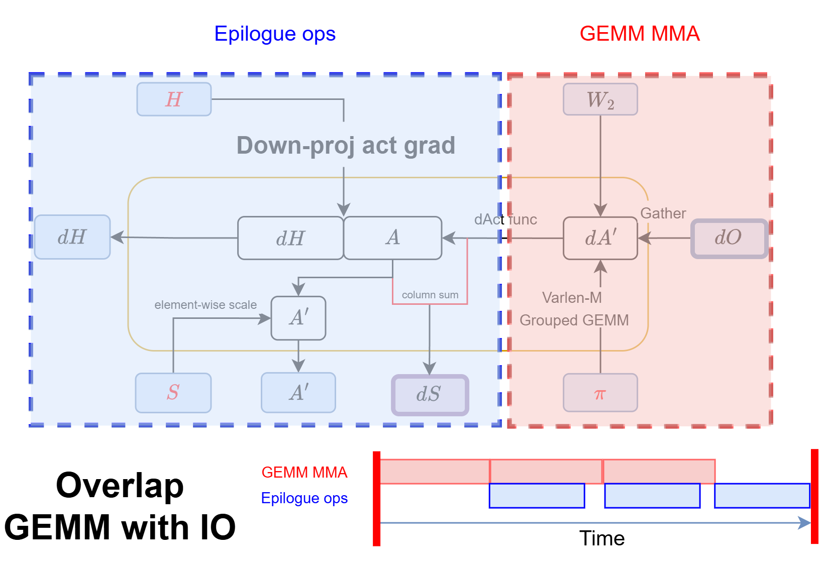
Figure: illustration of epilogue ops overlapped with GEMM MMA in SonicMoE's dH kernel.
In the following figure, we examine the hardware unit utilization of SonicMoE’s \(dH\) kernel with heavy epilogue (left column) or GEMM with normal epilogue store (right column) on Qwen3-235B-A22B-Thinking-2507 (\((T,d,n,E,K)=(32768,4096,1536,128,8)\)). The drop in MMA throughput is subproportional to the increase in epilogue IO costs:
- The \(dH\) kernel epilogue increases HBM traffic by 24% (6.33 to 7.86 GB).
- However, both the Tensor Core and Tensor Memory utilization only drop from 98% to 88% with the corresponding TFLOPS drop from 1213 to 1078 (11% decrease).
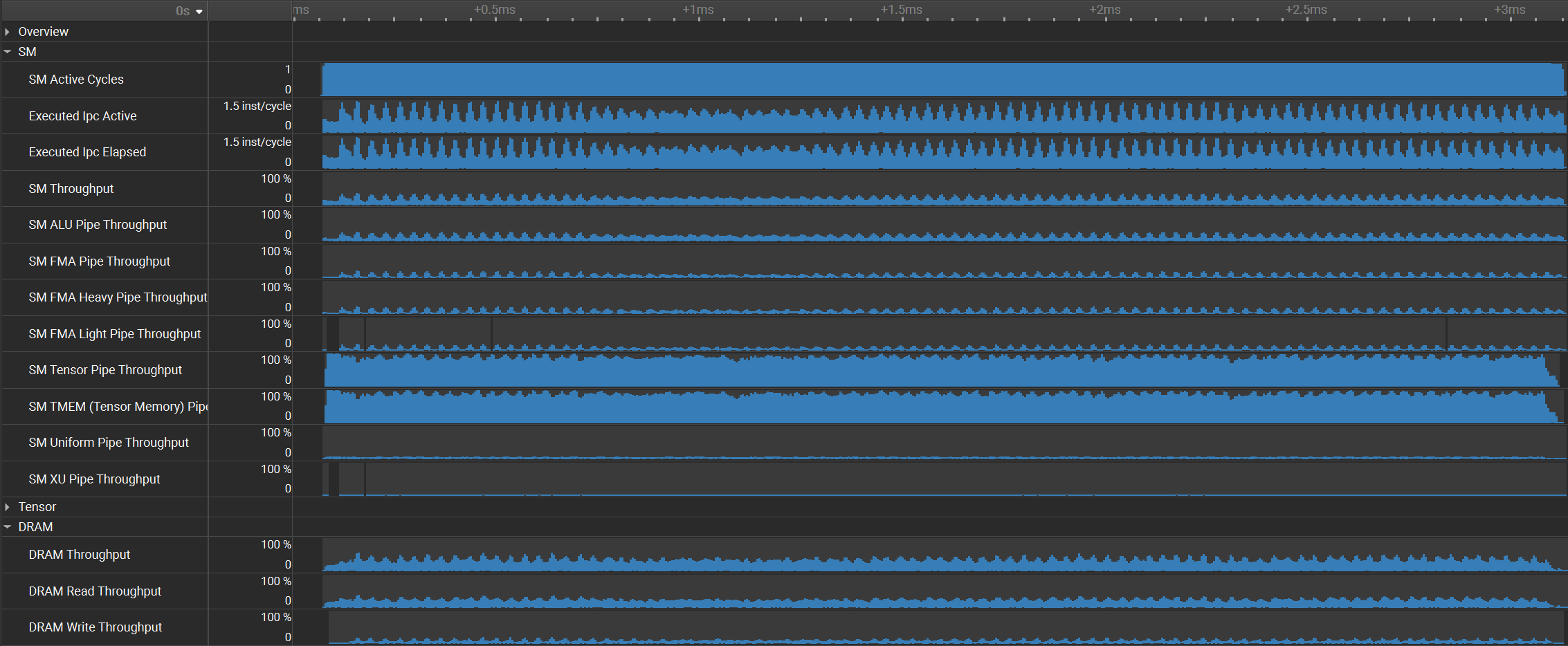
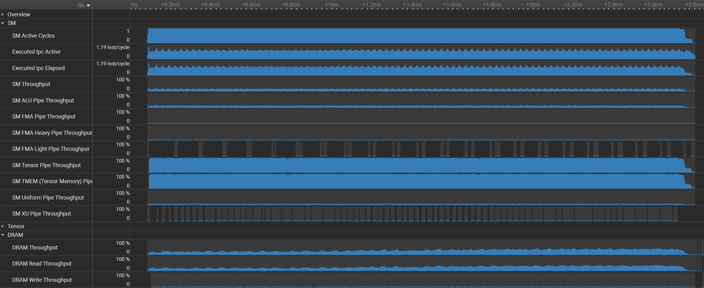
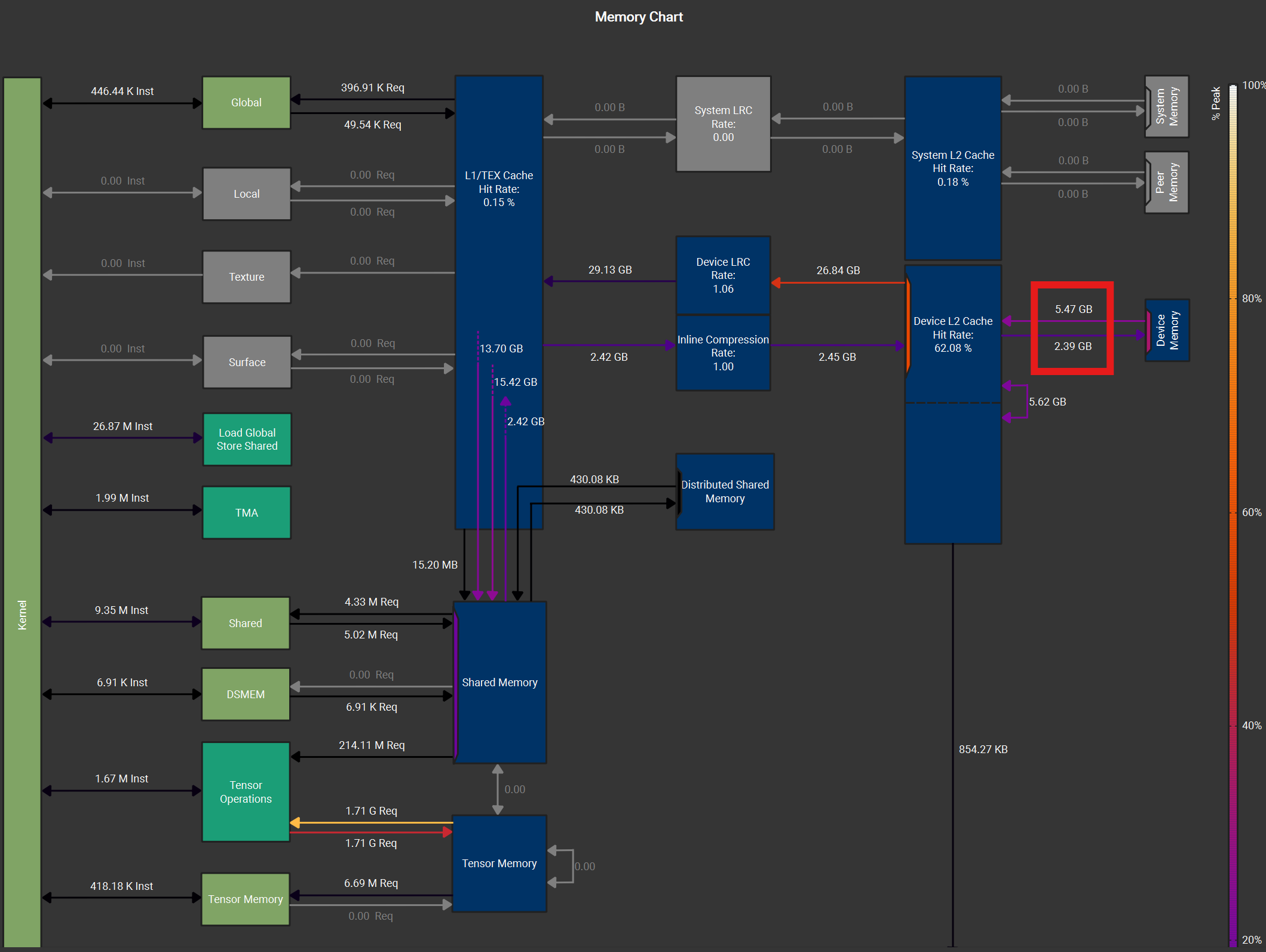
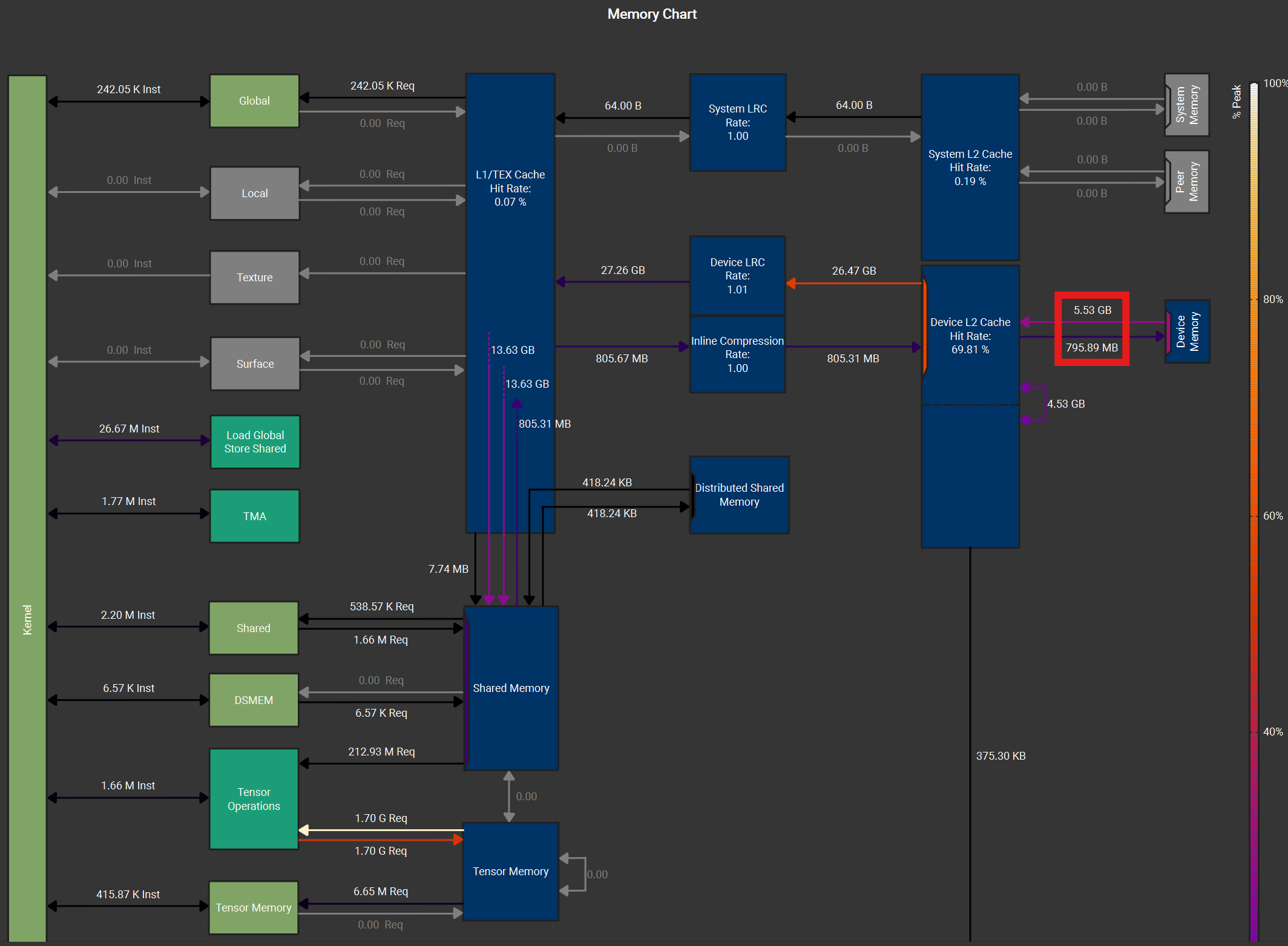
Figure: Nsight Compute Profiling of SonicMoE's dH kernel Grouped GEMM with 4 epilogue ops (left column) vs. Grouped GEMM alone (right column) of Qwen3-235B-A22B-Thinking-2507 (microbatch size=32k) on B300 GPUs. The top row is the achieved throughput of Tensor Pipe (MMA) and DRAM at kernel runtime, and the bottom row shows the transferred bytes on hardware units.
Overlapping IO with computation effectively absorbs the additional memory traffic, so the increase in IO cost does not translate proportionally into increased runtime.
5. Benchmark Results
We evaluate SonicMoE against multiple baselines on B300 GPUs. We benchmark the forward and backward pass of a single MoE layer with configurations adapted from open-source 7B to 685B MoE, and we then profile kernel-level time breakdown on 7B MoE specifically.
Forward and Backward TFLOPS of 6 Open-source MoE Configs
The figure below shows forward and backward TFLOPS across six real open-source MoE configurations, ranging from a 7B to a 685B MoE model.
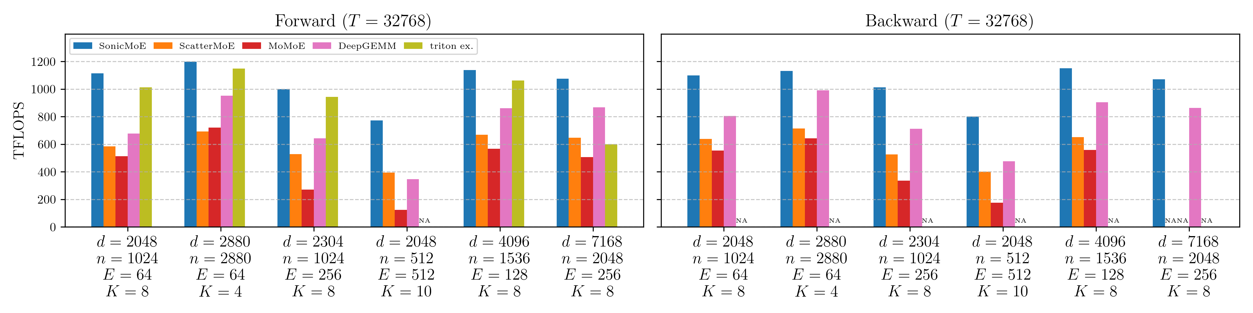
Figure: Forward (left) and backward (right) TFLOPS on B300 for 6 real MoE configurations. From left to right: OLMoE-1B-7B-0125, gpt-oss-20b, Kimi-Linear-48B-A3B-Base, Qwen3-Next-80B-A3B-Thinking, Qwen3-235B-A22B-Thinking-2507, and DeepSeek-V3.2-Exp. Triton official example does not support backward pass, nor K=10 for Qwen3-Next-80B forward pass.
Baselines:
| Baseline | Description |
|---|---|
| ScatterMoE | OpenLM Engine version (same kernel code, slightly different API). |
| MoMoE | Official implementation with shared experts disabled and expert bias adjustment removed. |
| DeepGEMM | DeepGEMM’s SM100 varlen-M and varlen-K BF16 Grouped GEMM, paired with a separate optimized gather kernel and torch.compile for all activation and expert aggregation kernels. This represents the throughput a practitioner would achieve by integrating DeepGEMM as a drop-in Grouped GEMM library. |
| Triton official example | Adapted from bench_mlp.py with expert parallelism disabled. |
Results:
SonicMoE consistently leads on all configurations. On average across 6 configs, SonicMoE achieves 54%/35% higher forward/backward TFLOPS than DeepGEMM baseline, and 21% higher forward TFLOPS than triton official example. SonicMoE has a decisive advantage (often achieving double TFLOPS) over the ScatterMoE and MoMoE baselines across all configs.
Profiling Time Breakdown
The runtime breakdown below makes the speedup concrete. The “gather \(X\)” segment in the forward pass and “gather \(dO\) and \(X\)” segment in the backward pass are absorbed into the GEMM bars for SonicMoE, and this constitutes one major source of speedup over the DeepGEMM-built baseline, which also has optimized Grouped GEMM but requires a separate gather kernel.
We note that although Triton official example has gather fusion and does not store \(H\) (as it is inference-oriented with no need of caching activation), SonicMoE is still faster for all three kernels during forward pass. This is because SonicMoE employs a faster Grouped GEMM implementation with the CLC tile scheduler and 2CTA MMA, and the expert aggregation kernel is heavily optimized. Please refer to the appendix for more details.
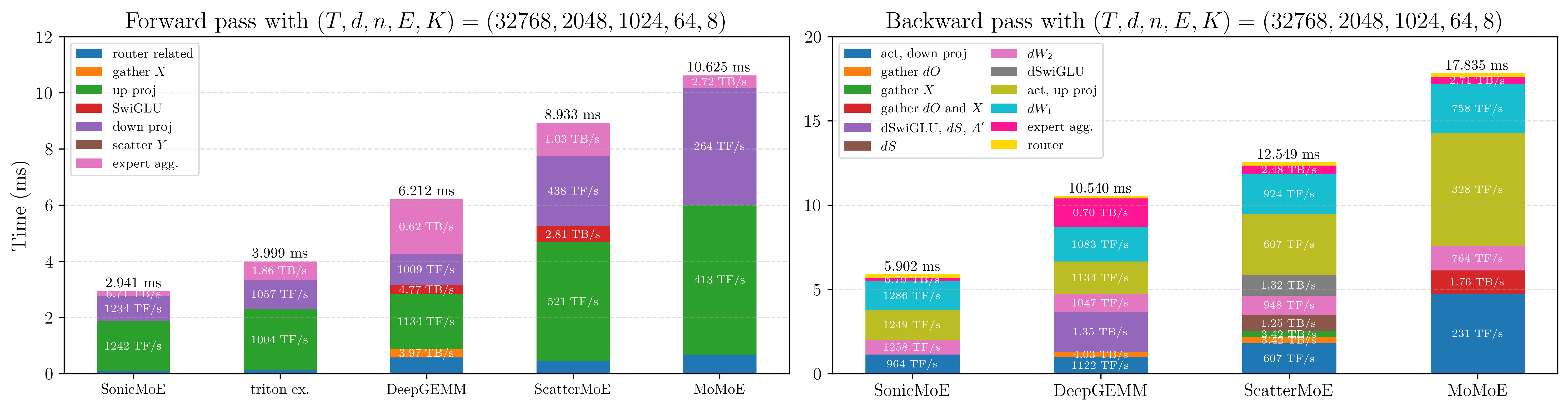
Figure: Runtime breakdown of SonicMoE vs baselines on B300 for a 7B OLMoE-sized MoE (T=32768, d=2048, n=1024, E=64, K=8). Detailed descriptions of other baselines can be found in the caption of Figure 5 of our arXiv paper. On this config, SonicMoE's major speedup comes from the gather fusion, and the faster GEMM delivers another 10% speedup. We abbreviate TFLOPS as "TF/s" in the figure.
Conclusion
SonicMoE started from a simple observation: the field is building MoEs that are more fine-grained and sparser with every generation, and existing kernels were not designed for that regime. Roughly 2 years from Mixtral to Kimi K2.5 represent a 9× increase in granularity and a 12× drop in activation ratio, and every step of that journey makes the arithmetic intensity worse and the activation memory larger. We need to re-visit our infrastructure design blueprint to embrace this MoE model trend, and SonicMoE is one of our answers.
-
Activation memory-efficient and IO-aware algorithm design. By redesigning the backward pass to avoid caching any \(O(TKd)\)-sized tensor, SonicMoE’s per-layer activation memory is independent of expert granularity — matching a dense model with the same activated parameter count, without any GEMM recomputation. The same algorithmic reordering eliminates multiple large HBM round-trips, and the remaining IO costs are largely hidden behind MMA computation through hardware asynchrony on both Hopper and Blackwell GPUs.
-
Extensible software abstraction with hardware-aware optimization. All of SonicMoE’s kernels are instances of one shared structure built on QuACK. This abstraction confines architecture-specific behavior to localized overrides while leaving the epilogue fusion logic and the GEMM interface untouched. This enables fast iteration for prototyping new model architectures and benchmarking new hardware features.
Future directions. The most immediate extension is expert parallelism: the IO-aware design principles transfer directly to the intra-node and inter-node setting, where network bandwidth is even more constraining than HBM. After that, we plan to add MXFP8 and MXFP4 support. Finally, the next GPU generation (Rubin) will bring new hardware primitives, and with the abstraction in place, we expect the port to require no more work than the Hopper-to-Blackwell migration did.
Citing this blogpost
If you find SonicMoE helpful in your research or development, please consider citing us:
@article{guo2025sonicmoe,
  title={SonicMoE: Accelerating MoE with IO and Tile-aware Optimizations},
  author={Guo, Wentao and Mishra, Mayank and Cheng, Xinle and Stoica, Ion and Dao, Tri},
  journal={arXiv preprint arXiv:2512.14080},
  year={2025}
}
References
[1] Yang, Haoqi, et al. “Faster moe llm inference for extremely large models.” arXiv preprint arXiv:2505.03531 (2025).
[2] Michael Diggin. “Implementing a Split-K Matrix Multiplication Kernel in Triton.” https://medium.com/@michael.diggin/implementing-a-split-k-matrix-multiplication-kernel-in-triton-7ad93fe4a54c
[3] NVIDIA CUTLASS Documentation. “Blackwell Cluster Launch Control.” https://docs.nvidia.com/cutlass/4.4.1/media/docs/cpp/blackwell_cluster_launch_control.html
[4] Modular. “Matrix Multiplication on NVIDIA’s Blackwell Part 3: The Optimizations Behind 85% of SOTA Performance.” https://www.modular.com/blog/matrix-multiplication-on-nvidias-blackwell-part-3-the-optimizations-behind-85-of-sota-performance
[5] PyTorch Blog. “Enabling Cluster Launch Control with TLX.” https://pytorch.org/blog/enabling-cluster-launch-control-with-tlx/
[6] Alex Armbuster. “How To Write A Fast Matrix Multiplication From Scratch With Tensor Cores.” https://alexarmbr.github.io/2024/08/10/How-To-Write-A-Fast-Matrix-Multiplication-From-Scratch-With-Tensor-Cores.html
[7] K.V. Nagesh. “NVIDIA Blackwell Architecture: A Deep Dive into the Next Generation of AI Computing.” https://medium.com/@kvnagesh/nvidia-blackwell-architecture-a-deep-dive-into-the-next-generation-of-ai-computing-79c2b1ce3c1b
Appendix
Below, we collect implementation comparisons and ablation studies that support the main text. We present a few ablation studies: cp.async vs. TMA gather4 for gather fusion, L2 cache locality analysis of gather fusion, and the design choice between GEMM + gather-and-sum vs. GEMM with scatter fusion + sum for expert aggregation.
Ablation Studies
cp.async vs. TMA gather4 for gather fusion
We first autotune on the best GEMM configs (tile shape, tile scheduler type, etc.) with cp.async, and then we switch in-place to TMA gather. In the following figure, we find that these two mechanisms deliver similar TFLOPS (diff < 2% for most cases). Nevertheless, we add whether to use TMA gather or cp.async gather as an autotunable configuration at kernel runtime.
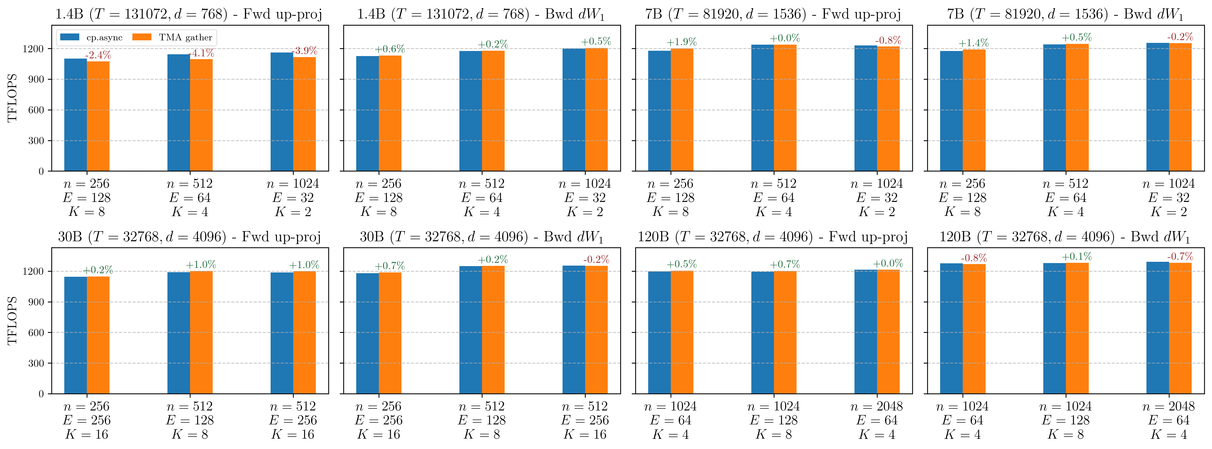
Figure: `cp.async` vs. TMA gather TFLOPS for forward pass up-proj (gather on M dim) and backward dW1 kernel (gather on K dim) kernels on B300 GPUs. Percentages indicate the relative TFLOPS difference of TMA gather over `cp.async`.
L2 Cache Locality with Gather Fusion
We compare the gather fusion against running a separate gather kernel to pre-arrange the inputs into a contiguous buffer before feeding into the Grouped GEMM kernel. The Nsight Compute memory charts below show a varlen-M Grouped GEMM kernel with gather fusion (left) and with pre-gathered contiguous inputs (right). Despite nearly identical L2->SMEM traffic (17.74 GB), the gather fusion (left figure) shows less HBM load traffic (2.20 vs 2.68 GB) and higher L2 cache hit rate (74.9% vs 66.3%).
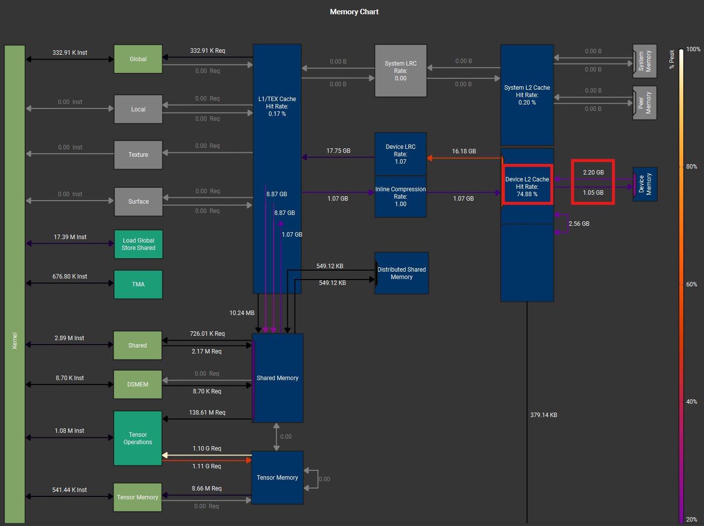
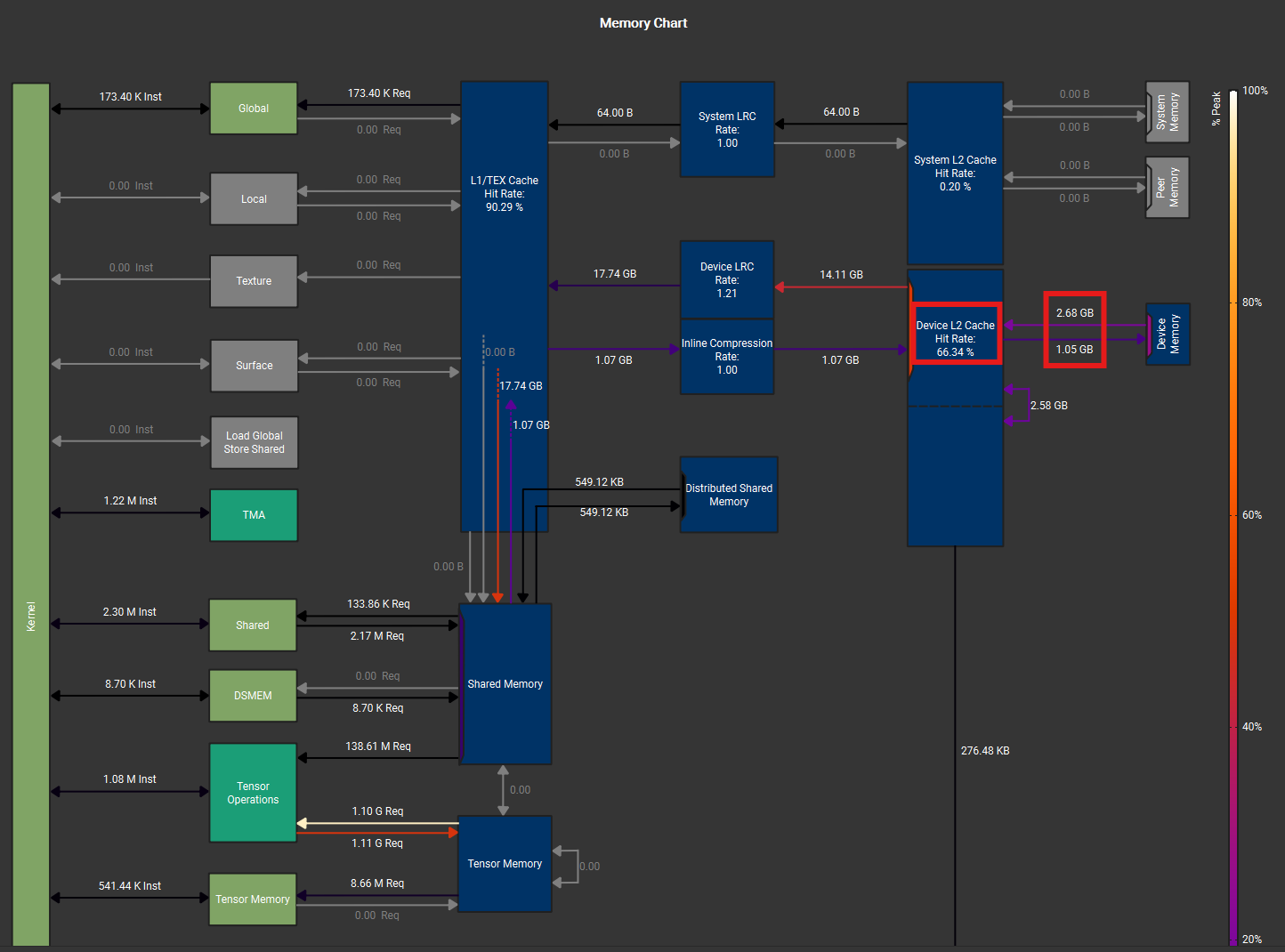
Figure: Nsight Compute memory chart for varlen-M Grouped GEMM during up-proj forward pass for MoE with size (T, d, n, E, K) = (32768, 2048, 512, 256, 32). Left: gather fusion with `cp.async`. Right: contiguous TMA load with pre-gathered inputs. Both use the same tile shape, scheduler configuration, and L2 swizzling pattern.
This is because gather fusion’s source tensor (\(X\) or \(dO\)) often has size \(T \times d\), which is \(K\times\) smaller than the pre-gathered tensor of size \(T\times K \times d\). As expert granularity increases, \(K\) grows proportionally, and the pre-gathered tensor can exceed the GPU’s L2 cache capacity (192 MB on B300). When this happens, the data request will miss L2 and be served from HBM. Gather fusion avoids this: it reads from the compact original tensor, which is more likely to stay resident in L2 cache.
This advantage compounds with expert granularity. Gathered \(X\) and gathered \(dO\), which are inputs to four of SonicMoE’s six Grouped GEMM kernels, are both \(O(TKd)\)-sized and grow linearly with \(K\). The figures below confirm the trend across three model families: as granularity increases (from left to right on each column), the contiguous path’s HBM load traffic grows faster and its L2 hit rate drops further relative to gather fusion.
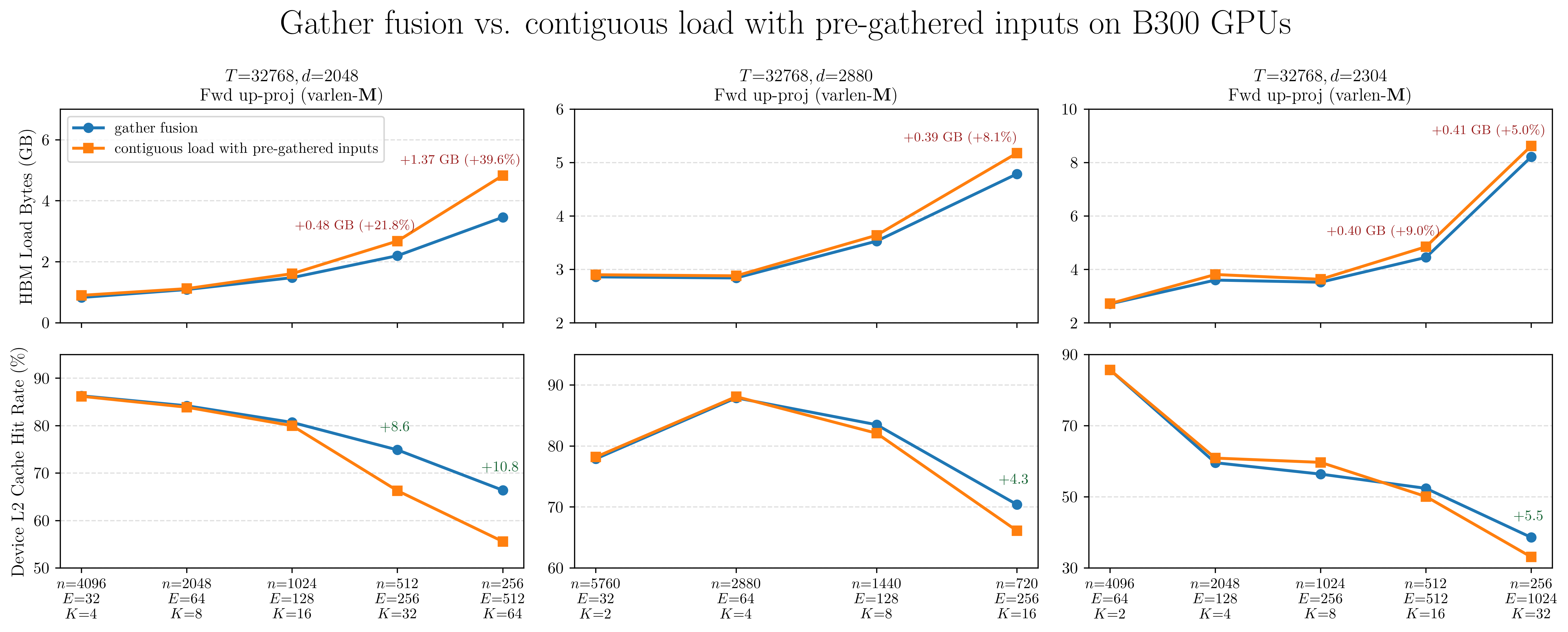
Figure: HBM load bytes (top row) and device L2 cache hit rate (bottom row) for gather fusion vs. contiguous load across varying expert granularity on B300 GPUs. Annotations on the top row show the absolute and relative HBM load increase of the contiguous path over gather fusion. Annotations on the bottom row show the L2 hit rate advantage of gather fusion.
Expert Aggregation Bandwidth
In SonicMoE’s expert aggregation kernel, each token will gather the Grouped GEMM results and sum over them in parallel. No GEMM is involved and this is a memory-bound kernel. The first version was implemented on CuteDSL, but we later switched to a pure Triton implementation due to the convenience of autotuning. This kernel achieves close-to-peak memory bandwidth on Hopper; here we validate its performance on Blackwell:
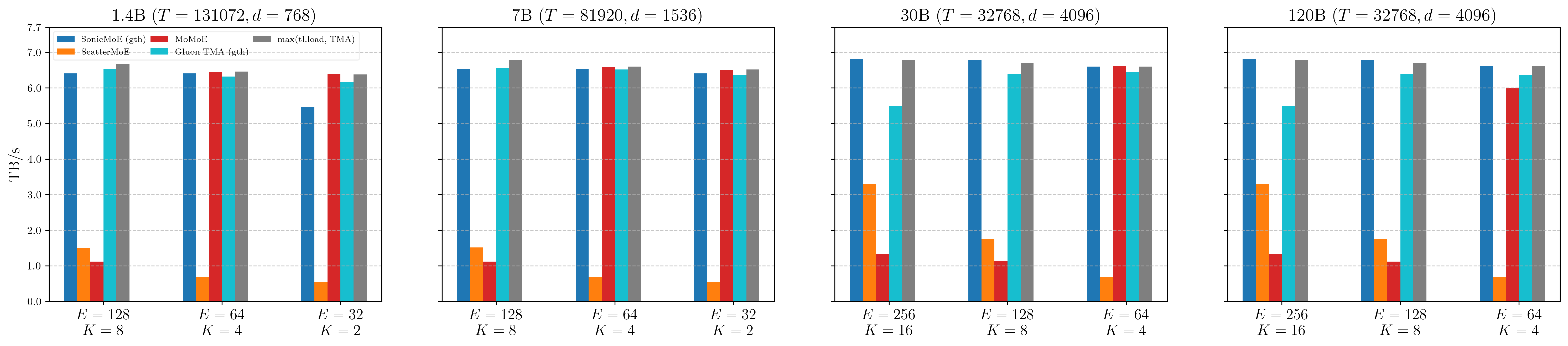
Figure: Expert aggregation kernel memory bandwidth on B300 across 1.4B, 7B, 30B, and 120B MoE configurations. SonicMoE's gather-and-sum kernel (blue) approaches the triton upper bound (grey, max of tl.load and TMA) at every scale.
Surprisingly, we find this Triton implementation still performs well enough on Blackwell GPUs (B300). This kernel surpasses 6.5 TB/s (85%+ peak) across most configs, achieving 98% of an optimized summation kernel on contiguous inputs. We also find this simple aggregation kernel outperforms the Gluon TMA gather-and-sum, adapted from Gluon official example implementation by 5% on average. This further suggests that gather with cp.async is not worse than TMA gather.
GEMM + gather-and-sum vs. GEMM with scatter + sum aggregation
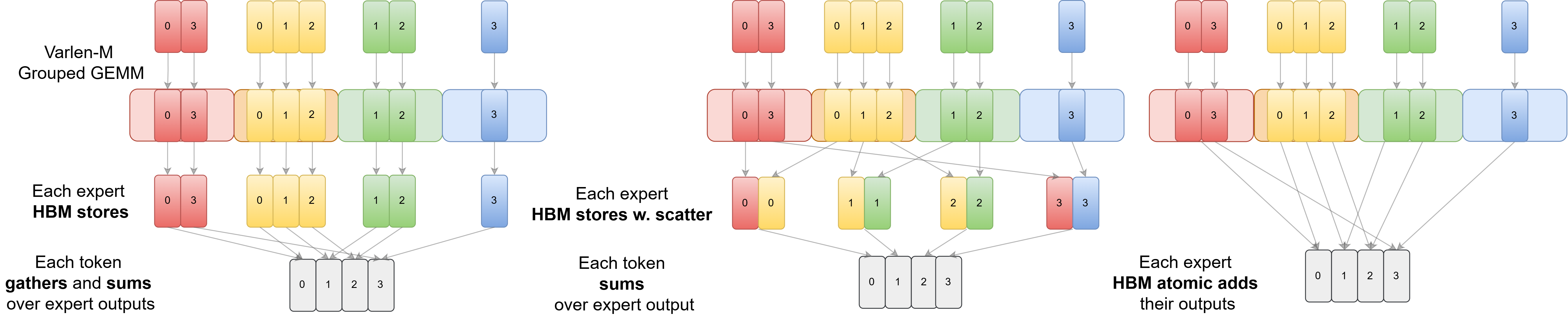
Figure: Possible strategies for storing the results and aggregating the results for each token. SonicMoE chooses the first strategy (left) in which each expert directly stores contiguously-packed outputs via TMA in the GEMM epilogue. In the expert aggregation kernel, each token gathers and sums over activated expert outputs. ScatterMoE and MoMoE (middle) choose to fuse HBM store with scatter in epilogue and launch a summation kernel afterwards. It is also possible to fuse atomic add in the epilogue to circumvent the requirement of an expert aggregation kernel as the right subfigure illustrated.
On Hopper GPUs, SonicMoE makes an unconventional design choice that we do not fuse scatter with GEMM. Instead, we perform this task alongside the aggregation. We previously ablated on Hopper GPUs and identified that the synchronous st.global PTX instruction required for scatter fusion on Hopper would degrade TFLOPS by 20% for fine-grained MoE configs.
An IO-aware design emerges only when algorithmic intent and hardware execution semantics are reasoned about together.
New Asynchronous Scatter Store Instructions on Blackwell
However, Blackwell introduces multiple asynchronous store instructions: (1) st.async.release.global and (2) TMA scatter4. The advantage of GEMM + gather-and-sum over GEMM w. scatter fusion + sum becomes less apparent as we no longer run into the synchronous IO issue for GEMM w. scatter fusion on Hopper. Even so, as we (1) do not observe major bandwidth degradation (0.98x) of gather-and-sum compared with contiguous summation kernel and (2) expect GEMM with TMA to be no slower than GEMM with TMA scatter4 or st.async, we do not change SonicMoE’s design choice on Blackwell.
We perform an ablation comparing varlen-M Grouped GEMM w. TMA + gather-and-sum against varlen-M Grouped GEMM w. TMA scatter + sum, adapting the official Triton Grouped GEMM example for both. The grouped gemm w. TMA + gth-and-sum approach stores Grouped GEMM results into a contiguously-packed tensor across all experts during the down-projection forward epilogue, where each token gathers and sums its corresponding expert outputs in a single fused operation. The grouped gemm w. TMA sct + sum approach instead scatters results via TMA during the epilogue and applies a separate contiguous summation kernel afterwards.
Disclaimer: the Grouped GEMM kernel in this ablation study is implemented with triton with fewer low-level optimizations (e.g. without 2CTA MMA) than SonicMoE’s Grouped GEMM, but it still provides insight on the relative performance comparison between GEMM w. TMA and GEMM w. TMA scatter4.
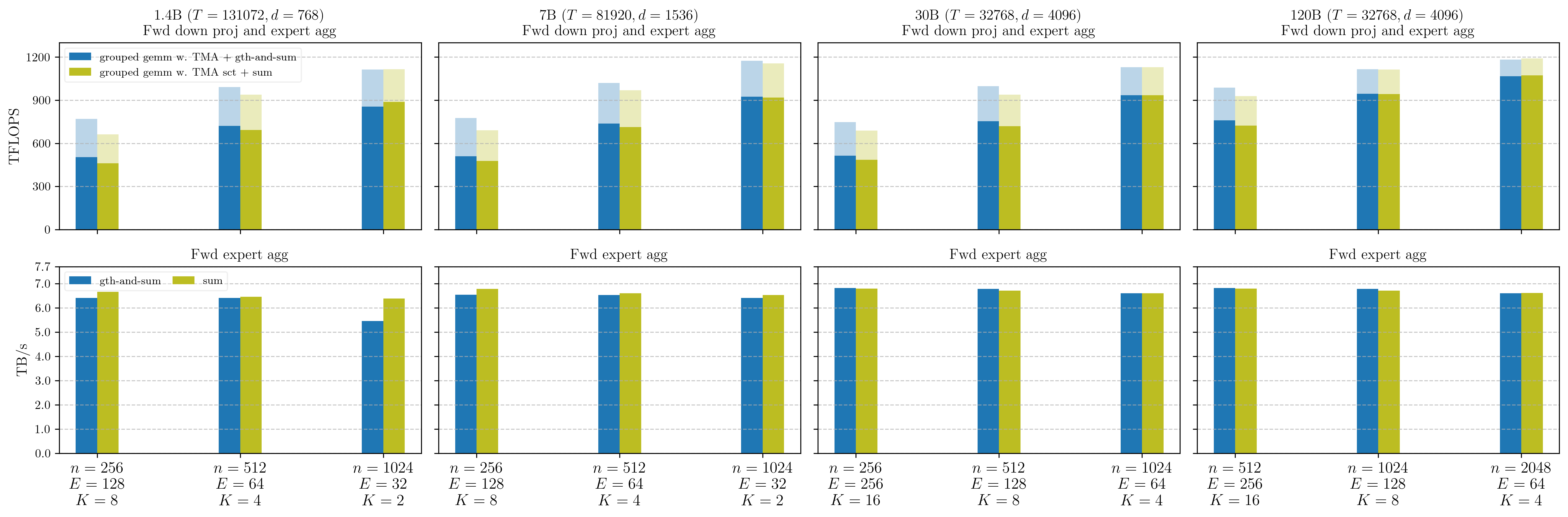
Figure: Throughput of varlen-M Grouped GEMM and expert aggregation kernel on B300 GPUs during forward pass. In the first row, we report the Grouped GEMM TFLOPS on transparent bars and the gemm-and-aggregation TFLOPS on opaque bars. In the second row, we compare the expert aggregation bandwidth between gather-and-sum and a contiguous sum kernel.
In the first row,
-
GEMM-only TFLOPS (transparent bars):
grouped gemm w. TMAstill has 5% higher TFLOPS thangrouped gemm w. TMA sct -
GEMM-and-aggregation TFLOPS (opaque bars):
grouped gemm w. TMA + gth-and-sumstill has 3% higher TFLOPS thangrouped gemm w. TMA sct + sum
In the second row, we already know that gth-and-sum only has 2% less bandwidth than sum.
Although this 3% gap is much smaller than the prior gap on Hopper GPUs (20%), it still validates SonicMoE’s design on Blackwell GPUs.